Case study: Groundwater monitoring

Author

Peter Ralph

Published

February 16, 2026

Wastewater in Eugene

Our wastewater (sewer plus stormwater) in Eugene and Springfield is treated by the Metropolitan Wastewater Management Commission, in part at the Biosolids Management Facility (see slideshow on that page).

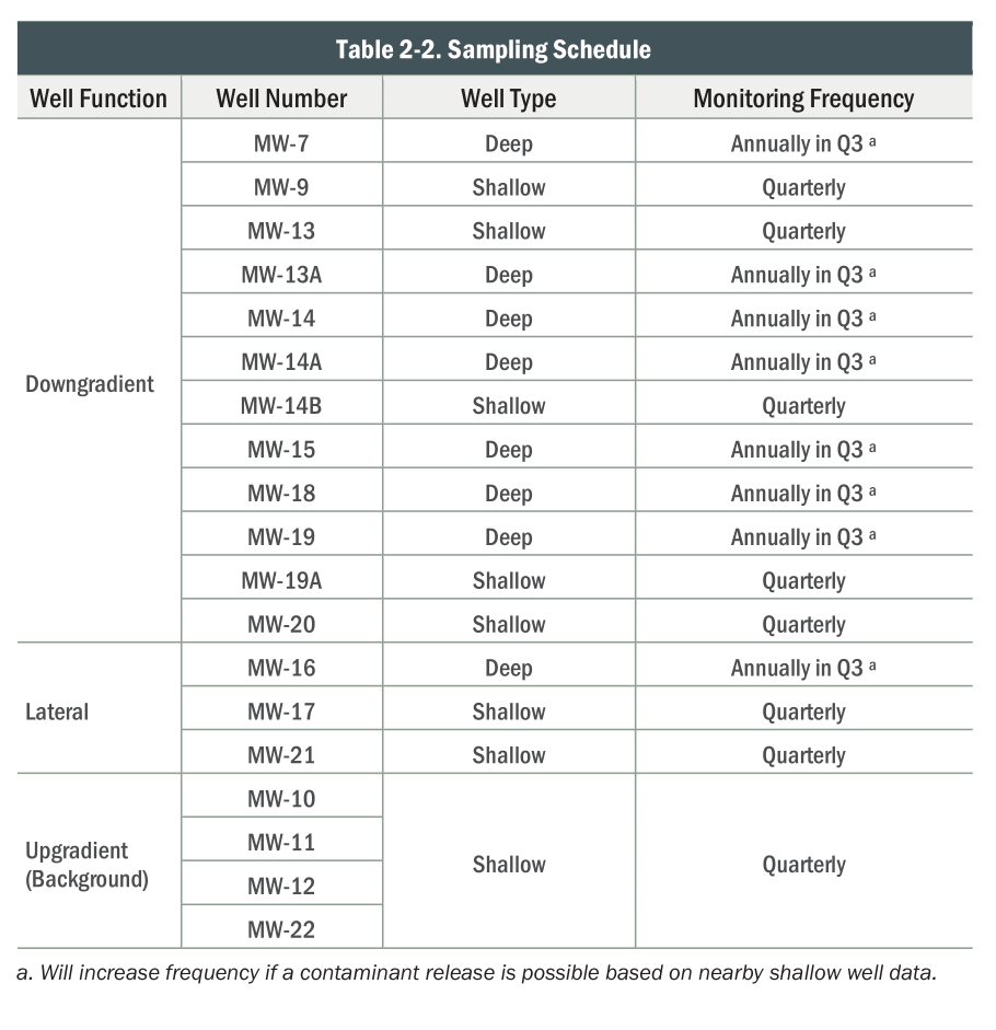
As part of their operating requirements, they monitor groundwater for potential contamination: in 26 monitoring wells, since 1988.

Their biggest question: how to best detect if the facility is affecting the groundwater?

Note: the MWMC is very much on top of this, and has no evidence of groundwater contamination. This is being presented for pedagogical purposes.

What is measured?

Table showing monitoring frequency for each well

Table showing variables that are monitored )

Overview of the data:

We’ve got:

Information about the wells: BMF_Well_details_2023_GWMP.csv
The actual measurements: Eugene_BiosolidsManagementFacility_GroundwaterData.csv

Set-up

import pandas as pd
import numpy as np
import plotnine as p9
import folium, pyproj

“Look at the data”, part 1

Game plan:

How many wells are there?
How many observations do we have from each, of what quantities, and over what time periods?
Where are the wells, and what do we know about them?

Preliminary answers above; but let’s check this!

Measurements

Measurements often run into detection limits; this is conveyed as “censoring status”.
well.name is the name of the location with the first year it was in operation appended

$ head data/Eugene_BiosolidsManagementFacility_GroundwaterData.csv | tr ',' '\t'
"well.name" "SampledDate"   "SampleNumber"  "ParameterName" "ParameterUnits"    "result"    "Method.Detection.Limit"    "Reporting.limit"   "censoring.status"  "Easting"   "Northing"
"MW-13-1988"    1988-01-25  "880050"    "Ammonia"   "mg/L"  0.1 NA  NA  "left.censored" 4218262.9   910814.599999998
"MW-13A-1988"   1988-01-25  "880052"    "Ammonia"   "mg/L"  0.1 NA  NA  "left.censored" 4218304.4   910813.2
"MW-14-1988"    1988-01-25  "880054"    "Ammonia"   "mg/L"  0.1 NA  NA  "left.censored" 4217612.3   910814.700000002
"MW-14A-1988"   1988-01-25  "880055"    "Ammonia"   "mg/L"  0.1 NA  NA  "left.censored" 4217622.5   910814.499999998
"MW-14B-1988"   1988-01-25  "880058"    "Ammonia"   "mg/L"  0.1 NA  NA  "left.censored" 4217612.9   910804.299999995
"MW-13-1988"    1988-01-25  "880050"    "Cadmium"   "µg/L"  1   NA  NA  "left.censored" 4218262.9   910814.599999998
"MW-13A-1988"   1988-01-25  "880052"    "Cadmium"   "µg/L"  1   NA  NA  "left.censored" 4218304.4   910813.2
"MW-14-1988"    1988-01-25  "880054"    "Cadmium"   "µg/L"  1   NA  NA  "left.censored" 4217612.3   910814.700000002
"MW-14A-1988"   1988-01-25  "880055"    "Cadmium"   "µg/L"  1   NA  NA  "left.censored" 4217622.5   910814.499999998

Pull in the data

gw = (
    pd.read_csv("data/Eugene_BiosolidsManagementFacility_GroundwaterData.csv")
    .convert_dtypes()
    .rename(columns=lambda x: x.replace(".", "_"))
    .assign(SampledDate = lambda df: pd.to_datetime(df['SampledDate']))
)
gw

	well_name	SampledDate	SampleNumber	ParameterName	ParameterUnits	result	Method_Detection_Limit	Reporting_limit	censoring_status	Easting	Northing
0	MW-13-1988	1988-01-25	880050	Ammonia	mg/L	0.1	<NA>	<NA>	left.censored	4218262.9	910814.6
1	MW-13A-1988	1988-01-25	880052	Ammonia	mg/L	0.1	<NA>	<NA>	left.censored	4218304.4	910813.2
2	MW-14-1988	1988-01-25	880054	Ammonia	mg/L	0.1	<NA>	<NA>	left.censored	4217612.3	910814.7
3	MW-14A-1988	1988-01-25	880055	Ammonia	mg/L	0.1	<NA>	<NA>	left.censored	4217622.5	910814.5
4	MW-14B-1988	1988-01-25	880058	Ammonia	mg/L	0.1	<NA>	<NA>	left.censored	4217612.9	910804.3
...	...	...	...	...	...	...	...	...	...	...	...
49552	MW-9-1996	2026-01-21	012126-01-03	WaterTableElevation	feet above mean sea level	361.44	<NA>	<NA>	not.censored	4217256.3	909769.9
49553	MW-19A-1988	2026-01-21	012126-01-04	WaterTableElevation	feet above mean sea level	361.72	<NA>	<NA>	not.censored	4217612.3	910354.1
49554	MW-13-2024	2026-01-21	012126-01-05	WaterTableElevation	feet above mean sea level	<NA>	<NA>	<NA>	not.censored	4218339.234158	910812.64945
49555	MW-14B-1988	2026-01-21	012126-01-06	WaterTableElevation	feet above mean sea level	360.56	<NA>	<NA>	not.censored	4217612.9	910804.3
49556	MW-20-1988	2026-01-21	012126-01-07	WaterTableElevation	feet above mean sea level	361.5	<NA>	<NA>	not.censored	4217582.6	909534.0

49557 rows × 11 columns

What’s measured?

gw.groupby("ParameterName")['result'].describe()

	count	mean	std	min	25%	50%	75%	max
ParameterName
Ammonia	3308.0	0.103789	0.03004	0.021	0.1	0.1	0.1	0.6
Cadmium	2508.0	0.390975	0.459542	0.0027	0.0075	0.2	1.0	5.0
ChemicalOxygenDemand	2489.0	8.962302	3.715514	3.6	5.0	10.0	10.0	96.0
Chloride	3316.0	5.562295	3.830561	0.5	3.8	5.0	6.9	49.0
Chromium	2510.0	2.394473	2.252434	0.045	0.511	2.0	5.0	56.0
Conductivity	3522.0	344.5477	143.069563	92.0	248.0	308.5	410.0	950.0
Copper	2520.0	2.897059	2.50814	0.039	0.3205	5.0	5.0	46.0
FecalColiform	3356.0	3.158522	25.10456	1.0	1.0	1.0	1.0	800.0
Lead	2502.0	2.105006	2.237623	0.002	0.0294	2.0	5.0	16.0
Nickel	2507.0	4.459762	4.080386	0.0087	0.456	5.0	10.0	13.0
Nitrate	3350.0	3.689657	2.205737	0.02	2.456	3.4	4.6	15.0
Temperature	223.0	13.675336	1.824945	8.6	12.6	13.5	14.8	18.8
TotalColiform	3346.0	6.614764	61.624235	1.0	1.0	1.0	1.0	2100.0
TotalDissolvedSolids	3358.0	231.526504	80.129682	60.0	180.0	214.0	270.0	880.0
TotalOrganicCarbon	2442.0	1.319935	1.039013	0.2	0.5	0.9	2.0	22.0
WaterTableElevation	3539.0	358.891123	3.812151	351.66	355.35	359.42	361.865	370.09
Zinc	2504.0	5.654278	4.790525	0.07	0.5735	10.0	10.0	20.0
pH	2250.0	6.945916	0.243518	5.94	6.81	7.0	7.1	8.4

How many things are measured?

Tabular form:

pd.crosstab(gw['well_name'], gw['ParameterName'])

ParameterName	Ammonia	Cadmium	ChemicalOxygenDemand	Chloride	Chromium	Conductivity	Copper	FecalColiform	Lead	Nickel	Nitrate	Temperature	TotalColiform	TotalDissolvedSolids	TotalOrganicCarbon	WaterTableElevation	Zinc	pH
well_name
MW-10-1983	44	47	45	47	47	47	47	47	47	47	43	0	44	45	43	48	47	0
MW-10-1996	132	87	86	131	86	138	87	132	86	86	131	17	131	131	86	139	86	118
MW-11-1983	47	48	48	47	48	49	48	49	48	48	48	0	46	49	45	49	48	0
MW-11-1996	130	85	86	130	85	140	84	130	84	84	131	14	130	132	84	140	83	117
MW-12-1983	46	47	47	48	47	46	47	48	47	47	48	0	47	48	44	48	47	0
MW-12-1996	125	86	83	126	86	140	85	124	84	85	126	14	125	126	83	142	85	122
MW-13-1988	141	97	98	140	97	149	97	147	97	97	141	1	144	142	93	152	97	80
MW-13-2018	26	27	26	26	28	32	30	27	28	29	27	2	27	26	27	31	29	32
MW-13-2024	7	6	6	6	6	7	6	7	6	6	6	7	7	6	6	7	6	7
MW-13A-1988	170	129	128	171	130	178	129	173	129	129	174	7	172	173	125	177	129	110
MW-14-1988	169	125	125	170	125	177	126	172	125	125	173	8	172	174	122	179	125	110
MW-14A-1988	179	132	132	179	132	184	133	181	132	132	182	6	181	181	128	187	132	116
MW-14B-1988	180	138	136	182	139	193	141	184	138	140	182	16	184	183	136	192	140	124
MW-15-1988	163	124	124	164	123	174	124	166	123	123	165	6	166	166	122	177	124	110
MW-16-1988	169	129	130	170	131	178	133	171	129	130	172	8	171	174	126	181	130	112
MW-17-1988	182	138	137	180	136	192	136	184	135	137	181	14	184	181	134	193	137	126
MW-18-1988	181	136	136	182	136	188	137	183	136	136	185	6	183	183	133	189	135	118
MW-19-1988	165	125	124	167	125	175	125	167	125	125	170	6	167	169	123	174	125	108
MW-19A-1988	175	135	131	176	134	197	135	180	134	133	179	19	179	176	130	201	134	136
MW-20-1988	183	136	134	179	138	199	139	189	139	136	186	18	189	182	135	202	135	137
MW-21-1988	178	136	135	179	136	187	137	180	136	136	179	15	180	181	133	185	136	121
MW-22-1988	172	133	130	172	133	184	133	175	133	135	173	19	176	175	129	186	133	117
MW-7-1983	45	48	48	46	48	49	48	40	48	48	46	0	45	48	45	49	48	0
MW-7-1996	123	78	78	123	78	126	78	123	78	78	123	5	123	126	78	128	78	106
MW-9-1983	47	48	48	47	48	48	48	48	48	48	47	0	44	48	45	49	48	0
MW-9-1996	129	88	88	128	88	145	87	129	87	87	132	15	129	133	87	141	87	123

When was each well used?

(
    pd.crosstab(gw['well_name'], gw['SampledDate'].dt.year)
    .reset_index()
    .melt(id_vars=['well_name'])
    .assign(year=lambda df: pd.to_numeric(df['SampledDate']))
    >>
    p9.ggplot(p9.aes(x='year', y='value', color='well_name'))
    + p9.geom_point() + p9.geom_line()
) + p9.theme(figure_size=(16,6))

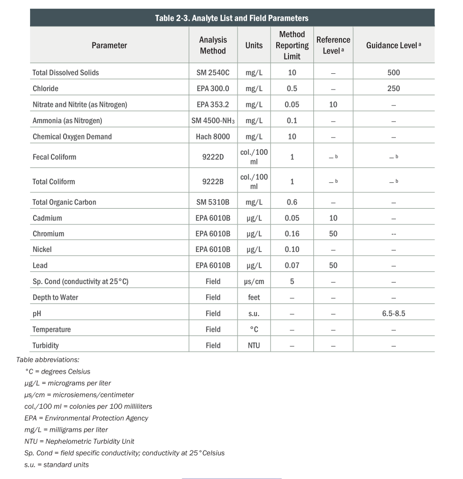
When was each thing measured?

(
    pd.crosstab(gw['ParameterName'], gw['SampledDate'].dt.year)
    .reset_index()
    .melt(id_vars=['ParameterName'])
    .assign(year=lambda df: pd.to_numeric(df['SampledDate']))
    >>
    p9.ggplot(p9.aes(x='year', y='value', color='ParameterName'))
    + p9.geom_point() + p9.geom_line()
    + p9.labs(y='number of measurements')
    + p9.theme(figure_size=(16,6))
)

Summary:

How many observations do we have from each, of what quantities, and over what time periods?

Exercise.

Where are the wells?

Well info

$ cat data/BMF_Well_details_2023_GWMP.csv | tr ',' '\t'
LocationName    well.orientation    well.depth.category screened.interval.feet
MW-7    downgradient    deep    42 to 52
MW-9    downgradient    shallow 15 to 25
MW-13A  downgradient    deep    30 to 50
MW-14   downgradient    deep    55 to 75
MW-14A  downgradient    deep    30 to 50
MW-14B  downgradient    shallow 10 to 25
MW-15   downgradient    deep    30 to 50
MW-18   downgradient    deep    30 to 50
MW-19   downgradient    deep    30 to 50
MW-19A  downgradient    shallow 10 to 25
MW-20   downgradient    shallow 10 to 25
MW-16   lateral deep    30 to 50
MW-17   lateral shallow 10 to 25
MW-21   lateral shallow 10 to 25
MW-10   upgradient  shallow 15 to 25
MW-11   upgradient  shallow 15 to 25
MW-12   upgradient  shallow 15 to 25
MW-22   upgradient  shallow 10 to 25
MW-13-2024  downgradient    shallow 10 to 25

Get per-well summaries from this

We’d like the location to be in the per-well table, so let’s pull this out of the “measurements” file first:

gw_wells = (
    gw.groupby(['well_name', 'Easting', 'Northing'])
    .aggregate(
        n = ('SampleNumber', lambda x: len(x)),
    )
    .reset_index()
    .assign(
        LocationName = lambda df: "MW-" + df['well_name'].str.extract("-([0-9A-Z]*)-"),
        FirstYear = lambda df: df['well_name'].str.extract("-([0-9A-Z]*)$")
    )
)    
gw_wells.loc[gw_wells['well_name'] == "MW-13-2024", 'LocationName'] = "MW-13-2024"

Well information

wells = pd.merge(
    (
        pd.read_csv("data/BMF_Well_details_2023_GWMP.csv")
        .convert_dtypes()
        .rename(columns=lambda x: x.replace(".", "_"))
    ),
    gw_wells, how='outer', on='LocationName'
)
wells

	LocationName	well_orientation	well_depth_category	screened_interval_feet	well_name	Easting	Northing	n	FirstYear
0	MW-10	upgradient	shallow	15 to 25	MW-10-1983	4219307.315854	909474.081725	735	1983
1	MW-10	upgradient	shallow	15 to 25	MW-10-1996	4217879.6	908303.2	1890	1996
2	MW-11	upgradient	shallow	15 to 25	MW-11-1983	4217171.326475	908754.90989	765	1983
3	MW-11	upgradient	shallow	15 to 25	MW-11-1996	4217227.5	908744.7	1869	1996
4	MW-12	upgradient	shallow	15 to 25	MW-12-1983	4219118.324783	908681.318636	752	1983
5	MW-12	upgradient	shallow	15 to 25	MW-12-1996	4219546.5	908262.3	1847	1996
6	MW-13	<NA>	<NA>	<NA>	MW-13-1988	4218262.9	910814.6	2010	1988
7	MW-13	<NA>	<NA>	<NA>	MW-13-2018	4218262.9	910814.6	480	2018
8	MW-13-2024	downgradient	shallow	10 to 25	MW-13-2024	4218339.234158	910812.64945	115	2024
9	MW-13A	downgradient	deep	30 to 50	MW-13A-1988	4218304.4	910813.2	2533	1988
10	MW-14	downgradient	deep	55 to 75	MW-14-1988	4217612.3	910814.7	2502	1988
11	MW-14A	downgradient	deep	30 to 50	MW-14A-1988	4217622.5	910814.5	2629	1988
12	MW-14B	downgradient	shallow	10 to 25	MW-14B-1988	4217612.9	910804.3	2728	1988
13	MW-15	downgradient	deep	30 to 50	MW-15-1988	4217592.3	909964.4	2444	1988
14	MW-16	lateral	deep	30 to 50	MW-16-1988	4217592.7	909113.7	2544	1988
15	MW-17	lateral	shallow	10 to 25	MW-17-1988	4219020.1	910333.0	2707	1988
16	MW-18	downgradient	deep	30 to 50	MW-18-1988	4217912.6	910784.0	2683	1988
17	MW-19	downgradient	deep	30 to 50	MW-19-1988	4217612.7	910364.2	2465	1988
18	MW-19A	downgradient	shallow	10 to 25	MW-19A-1988	4217612.3	910354.1	2684	1988
19	MW-20	downgradient	shallow	10 to 25	MW-20-1988	4217582.6	909534.0	2756	1988
20	MW-21	lateral	shallow	10 to 25	MW-21-1988	4218063.0	908984.0	2670	1988
21	MW-22	upgradient	shallow	10 to 25	MW-22-1988	4218563.1	908764.3	2608	1988
22	MW-7	downgradient	deep	42 to 52	MW-7-1983	4217236.222717	910903.762698	749	1983
23	MW-7	downgradient	deep	42 to 52	MW-7-1996	4217291.5	910895.9	1730	1996
24	MW-9	downgradient	shallow	15 to 25	MW-9-1983	4217197.302791	909779.024971	759	1983
25	MW-9	downgradient	shallow	15 to 25	MW-9-1996	4217256.3	909769.9	1903	1996

Mapping

Let’s use folium. Looking at the documentation, we need a location in “Latitude and Longitude of Map (Northing, Easting)”.

Easting and Northing coordinates are provided in the ESPG: 2270 Coordinate Reference System (NAD83 / Oregon South (ft))

So first: find the center of the well locations, and project it to lat/long.

def transform(easting, northing):
    crs = pyproj.CRS.from_epsg(2270)
    latlon = pyproj.CRS(proj='latlon', datum='WGS84')
    transformer = pyproj.Transformer.from_crs(crs, latlon)
    y, x = transformer.transform(easting, northing)
    return (x, y)

center = transform(wells['Easting'].mean(), wells['Northing'].mean())
center

(44.132343700797044, -123.17902808886248)

The wells:

folium.Map(location=center, zoom_start=16)

Make this Notebook Trusted to load map: File -> Trust Notebook

Let’s get some more info on that:

After some iteration:

import matplotlib

def add_marker(m, row=None, tooltip=None, location=None, **kwargs):
    defaults = {
        'radius': 10,
        'fill_color': "orange",
        'fill_opacity': 0.4,
        'color': 'black',
        'weight': 1
    }
    defaults.update(kwargs)
    if location is None:
        location = transform(row.Easting, row.Northing)
    if tooltip is None and row is not None:
        tooltip = row.LocationName
    return folium.CircleMarker(
        location=location,
        tooltip=tooltip,
        **defaults
    ).add_to(m)

def make_colormap(x, xmin=None, xmax=None, mapname='viridis'):
    cmap = matplotlib.colormaps[mapname]
    if xmin is None:
        xmin = np.min(x)
    if xmax is None:
        xmax = np.max(x)
    assert xmax > xmin, f"Must have xmin < xmax (got {xmin}, {xmax})."
    def f(x):
        colors = cmap((x - xmin)/(xmax - xmin))
        if isinstance(colors, tuple):
            colors = [colors]
        return [matplotlib.colors.to_hex(u) for u in colors]
    return f

well_bbox = (
    transform(wells['Easting'].min(), wells['Northing'].min()),
    transform(wells['Easting'].min(), wells['Northing'].max()),
    transform(wells['Easting'].max(), wells['Northing'].max()),
    transform(wells['Easting'].max(), wells['Northing'].min()),
)
def add_legend(m, colors, k=8, title=None):
    dy = (well_bbox[1][0] - well_bbox[0][0])/k
    pos = list(well_bbox[2])
    def text(pos, label):
        folium.Marker(
            pos,
            icon=folium.DivIcon(
                icon_size=(100,30),
                icon_anchor=(-15,15),
                html=f'<div style="font-size: 15pt">{label}</div>',
            )
        ).add_to(m)        
    if title is not None:
        text(pos, title)
        pos[0] -= dy
    for n in colors:
        add_marker(m, location=pos, fill_color=colors[n]).add_to(m)
        label = n if type(n) is str else 'NA'
        text(pos, label)
        pos[0] -= dy

Well orientation:

orientation_colors = {
    'upgradient' : "#66c2a5",
    'downgradient' : "#8da0cb",
    'lateral' : "#fc8d62",
    pd.NA : "#666666",
}

m = folium.Map(location=center, zoom_start=16)
add_legend(m, orientation_colors)
for r in wells.itertuples():
    add_marker(m, r,
        fill_color=orientation_colors[r.well_orientation],
    )

m

Make this Notebook Trusted to load map: File -> Trust Notebook

Well depth:

depth_colors = {
    'shallow' : "#7fc97f",
    'deep' : "#fdc086",
    pd.NA : "#666666",
}

m = folium.Map(location=center, zoom_start=16)
add_legend(m, depth_colors)
for r in wells.itertuples():
    add_marker( m, r,
        fill_color=depth_colors[r.well_depth_category],
    )

m

Make this Notebook Trusted to load map: File -> Trust Notebook

Summary

Where are the wells, and what do we know about them?

Exercise

“Look at the data”, part 2

Game plan:

Do the measurements differ most:
- between wells?
- between types of well? (up/downgradient, shallow/deep)
- between years?
- between seasons?
- all/some of the above?
Do nearby wells get similar measurements?

All the data, from 20,000 feet

(
    p9.ggplot(gw, p9.aes(x="SampledDate", y="result", color='well_name'))
    + p9.geom_line() + p9.geom_point(size=0.2, alpha=0.25)
    + p9.facet_grid(rows="ParameterName", scales='free_y')
) + p9.theme(figure_size=(8,24))

/home/peter/micromamba/envs/ds435/lib/python3.13/site-packages/plotnine/layer.py:374: PlotnineWarning: geom_point : Removed 7 rows containing missing values.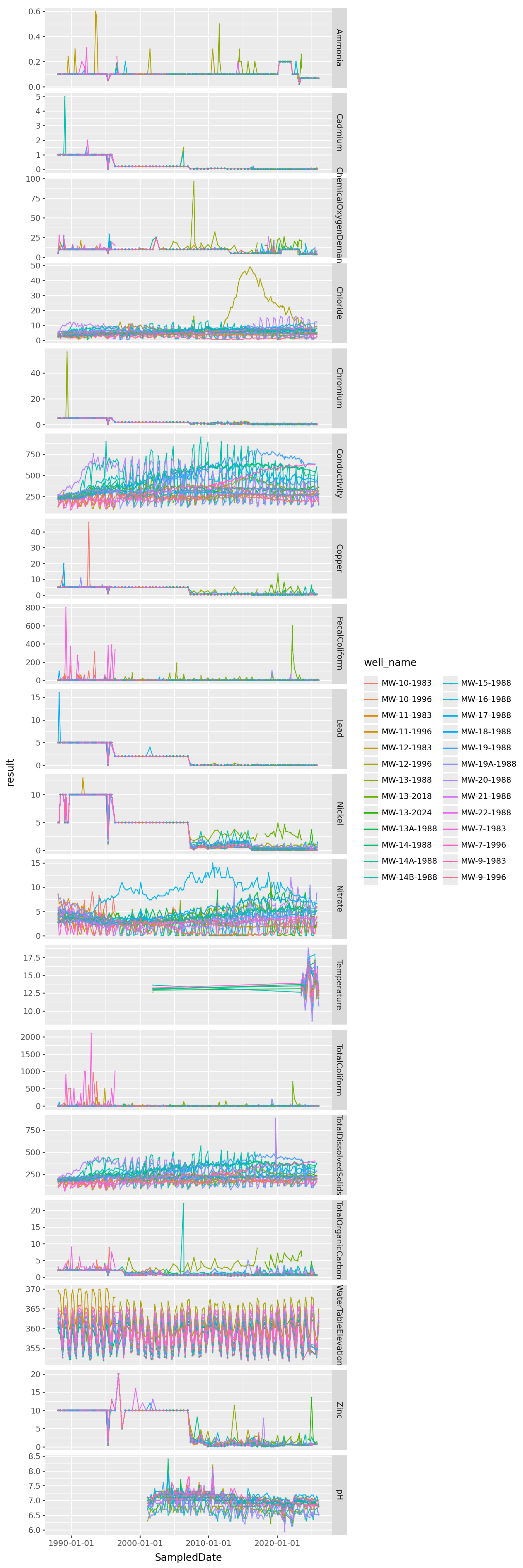

Observations?

What features do we see here and what do those features suggest doing?

Exercise:

Filter out the obvious outliers (eg Chromium, can’t tell what’s going on).
Which variables are most important to the audience of the report?
Consider removing wells or variables for which we don’t have complete observations: for instance, Temperature.
Conductivity:
- does the location relative to the plant,
- or type of well
- impact whether it’s increasing/decreasing long term,
- or whether it’s oscilating.
Are the oscillations in various variables always going along with water level/season?
Chloride: what happened with that one well that had very large values for a while?

Set-up:

Let’s add well categories to the measurement data:

gw = pd.merge(
    gw,
    wells.loc[:,('well_name', 'well_orientation', 'well_depth_category')],
    how='left',
    on='well_name'
)
gw.head()

	well_name	SampledDate	SampleNumber	ParameterName	ParameterUnits	result	Method_Detection_Limit	Reporting_limit	censoring_status	Easting	Northing	well_orientation	well_depth_category
0	MW-13-1988	1988-01-25	880050	Ammonia	mg/L	0.1	<NA>	<NA>	left.censored	4218262.9	910814.6	<NA>	<NA>
1	MW-13A-1988	1988-01-25	880052	Ammonia	mg/L	0.1	<NA>	<NA>	left.censored	4218304.4	910813.2	downgradient	deep
2	MW-14-1988	1988-01-25	880054	Ammonia	mg/L	0.1	<NA>	<NA>	left.censored	4217612.3	910814.7	downgradient	deep
3	MW-14A-1988	1988-01-25	880055	Ammonia	mg/L	0.1	<NA>	<NA>	left.censored	4217622.5	910814.5	downgradient	deep
4	MW-14B-1988	1988-01-25	880058	Ammonia	mg/L	0.1	<NA>	<NA>	left.censored	4217612.9	910804.3	downgradient	shallow

Outliers?

Here’s Chromium:

(
    gw
    .query("ParameterName == 'Chromium'")
    >> p9.ggplot(p9.aes(x="SampledDate", y="result", color="well_depth_category", group="well_name"))
    + p9.geom_line() + p9.geom_point(size=0.5, alpha=0.5)
) + p9.theme(figure_size=(9,4))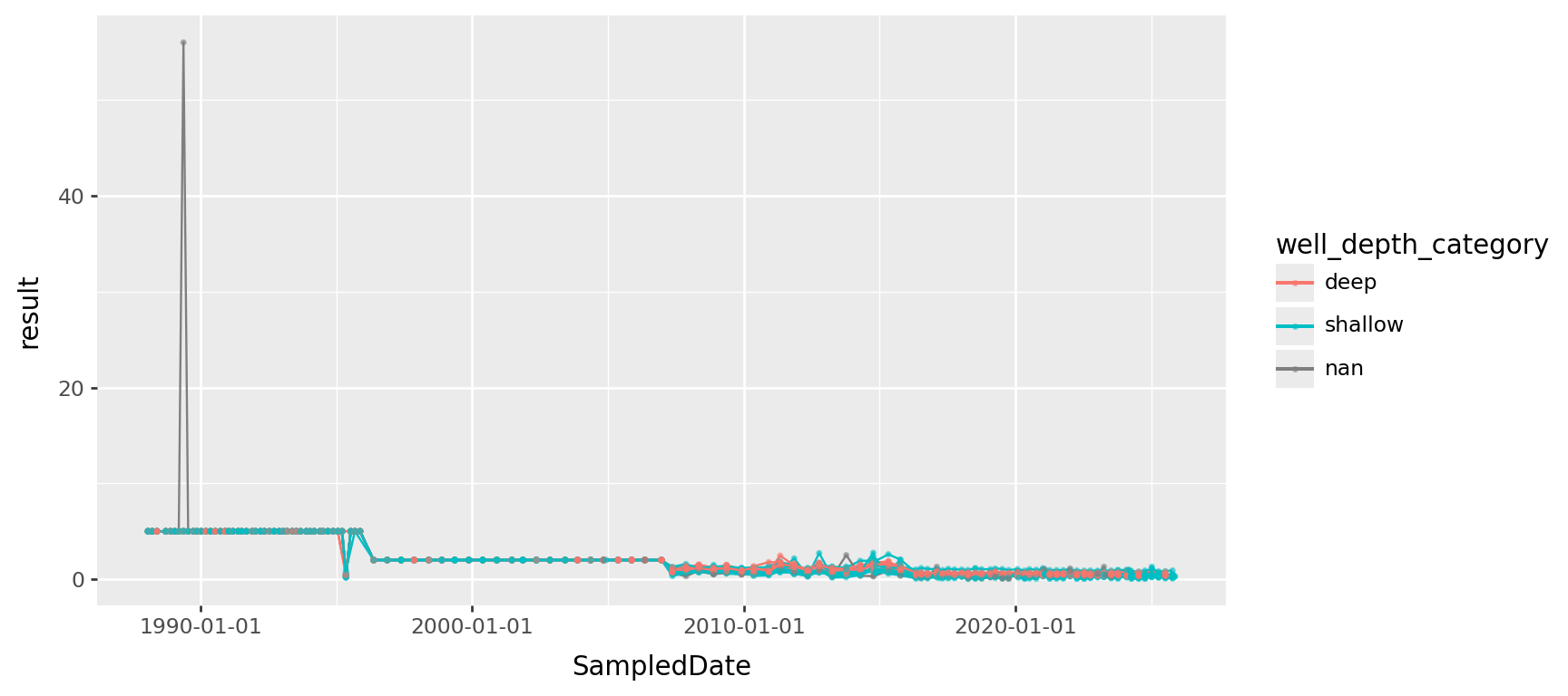

Ways to deal with outliers in visualization

Change the axis limits to zoom in on what you want.
Transform the variable (e.g., with log).
Programatically decide which ones are outliers and remove them.

Either the second or third methods sets you up for downstream analysis.
A transformation is better if it gives you “the right scale to look at the data on”.
The third method is good if you think the “outliers” are produced by some other process that is not of interest (for instance, measurement error).
A good generic way to do (3) is by computing \(z\) scores: z = (value - center)/scale.

Chromium, transformed

(
    gw
    .query("ParameterName == 'Chromium'")
    >> p9.ggplot(p9.aes(x="SampledDate", y="result", color="well_depth_category", group="well_name"))
    + p9.geom_line() + p9.geom_point(size=0.5, alpha=0.5)
    + p9.labs(title="Chromium", y="concentration (µg/L)")
    + p9.scale_y_log10()
) + p9.theme(figure_size=(9,4))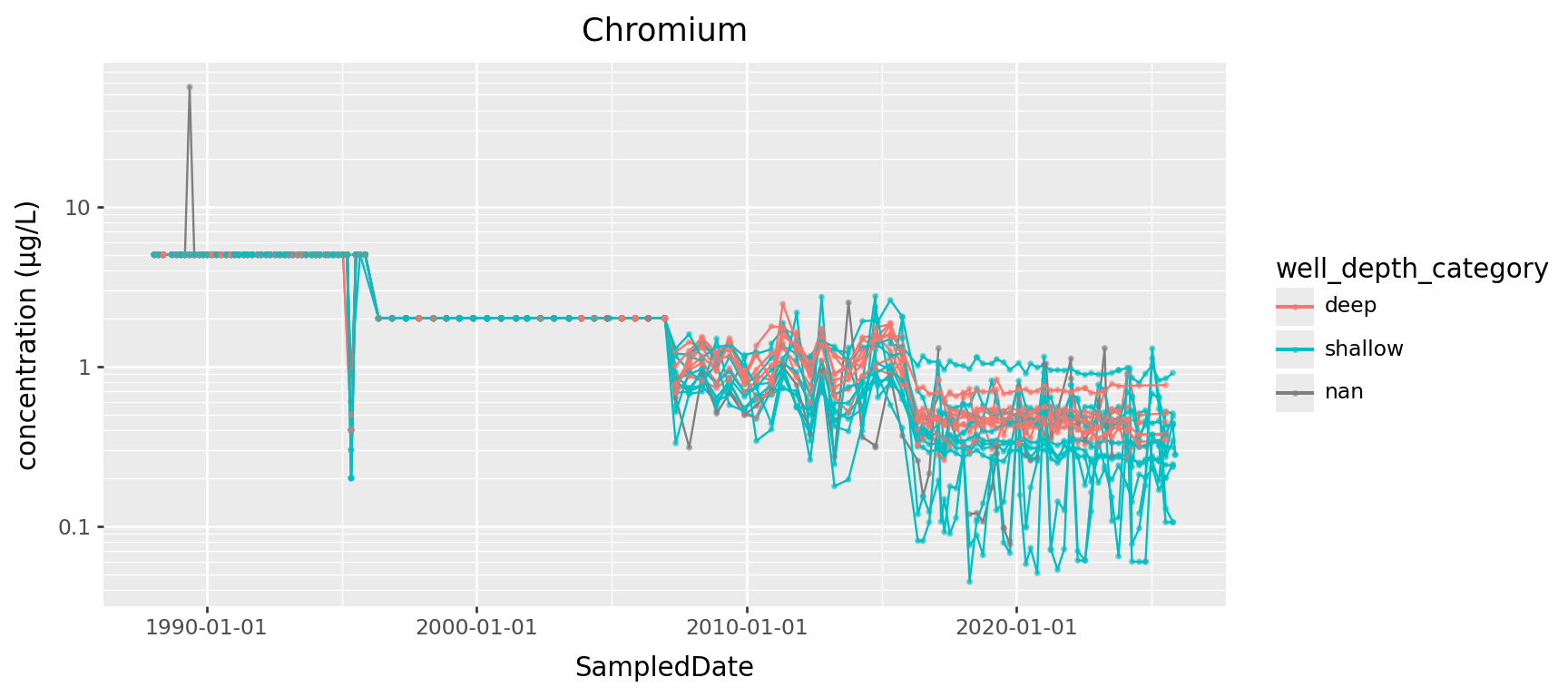

Chromium, “identifying outliers”?

z = (value - center) / scale

Question: what to use for “center” and “scale”? Median+IQR or mean+SD? Within groups? Which groups?

Definitely group by year in this case, since things change.
Usually I’d prefer “median and IQR”, but for many years the IQR is zero.

chromium = (
    gw.query("ParameterName == 'Chromium'")
    .assign(
        mean = lambda df: df['result'].groupby(df['SampledDate'].dt.year).transform('mean'),
        std = lambda df: df['result'].groupby(df['SampledDate'].dt.year).transform('std'),
        z = lambda df: (df['result'] - df['mean']) / ( df['std'] + (df['std'] == 0) ),
    )
)
chromium >> p9.ggplot(p9.aes(x='z')) + p9.geom_histogram(bins=40)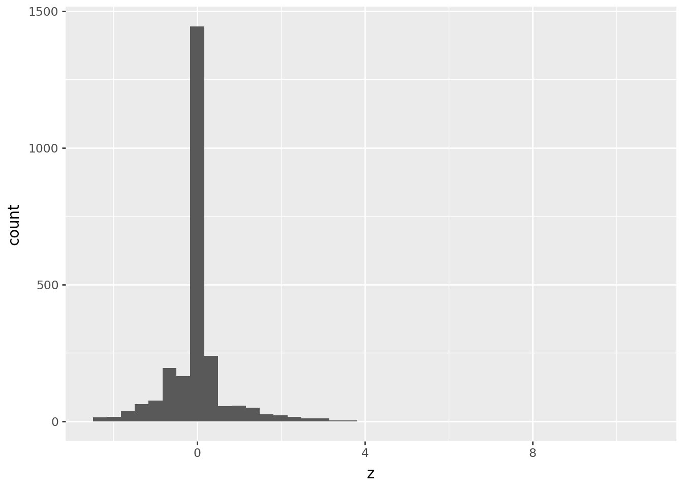

How’s that look?

The cutoff for “outlier” in terms of \(z\) scores should always be made looking at the data, but often between 3 and 5 is good, if this is a reasonable approach.

p1 = (
    chromium
    >>
    p9.ggplot(p9.aes(x="SampledDate", y="result", group="well_name"))
    + p9.geom_line(alpha=0.5)
    + p9.geom_point(mapping=p9.aes(color="z.abs() > 5"))
    + p9.labs(title="Chromium", y="concentration (µg/L)")
)
p2 = (
    chromium
    .query("abs(z) < 5")
    >>
    p9.ggplot(p9.aes(x="SampledDate", y="result", group="well_name"))
    + p9.geom_line(alpha=0.5)
    + p9.geom_point()
    + p9.labs(title="Chromium", y="concentration (µg/L)")
)
(p1 / p2)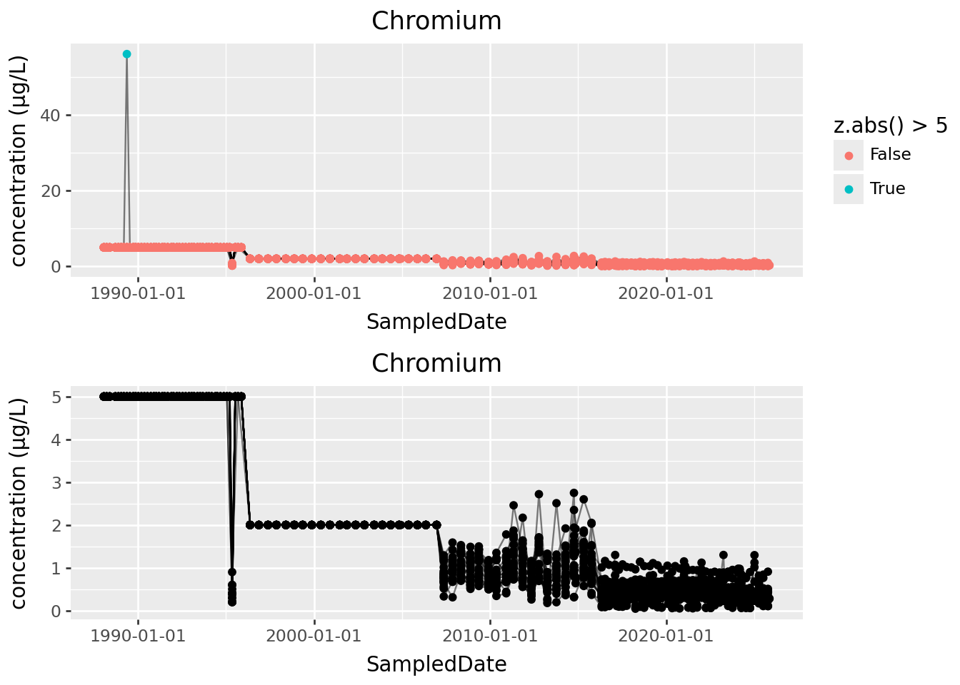

All the heavy metals

metals = ["Cadmium", "Chromium", "Copper", "Lead", "Nickel", "Zinc"]
(
    gw
    .loc[gw['ParameterName'].isin(metals), :]
    >> p9.ggplot(p9.aes(x="SampledDate", y="result", color="well_orientation", group="well_name"))
    + p9.geom_line() + p9.geom_point(size=0.5, alpha=0.5)
    + p9.scale_y_log10()
    + p9.facet_grid(rows="ParameterName")
) + p9.theme(figure_size=(9,12))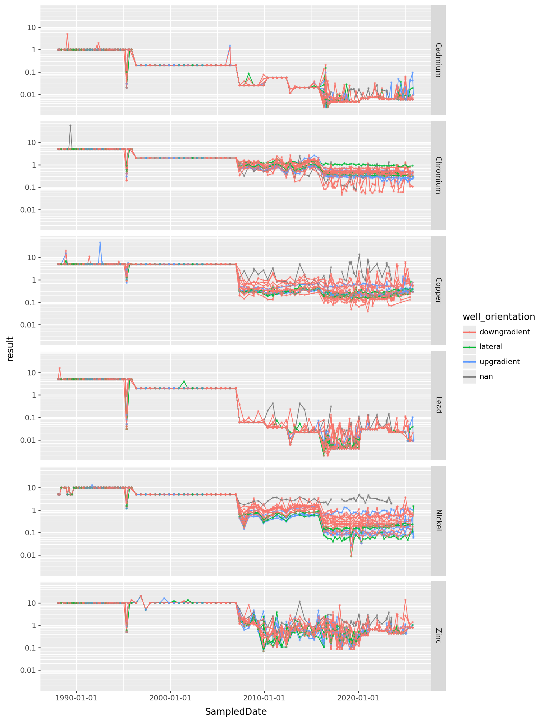

All the heavy metals, since 2016

(
    gw
    .loc[(gw['ParameterName'].isin(metals)) & (gw['SampledDate'].dt.year >= 2016), :]
    >> p9.ggplot(p9.aes(x="SampledDate", y="result", color="well_orientation", group="well_name"))
    + p9.geom_line() + p9.geom_point(size=0.5, alpha=0.5)
    + p9.scale_y_log10()
    + p9.facet_grid(rows="ParameterName", scales="free_y")
) + p9.theme(figure_size=(9,12))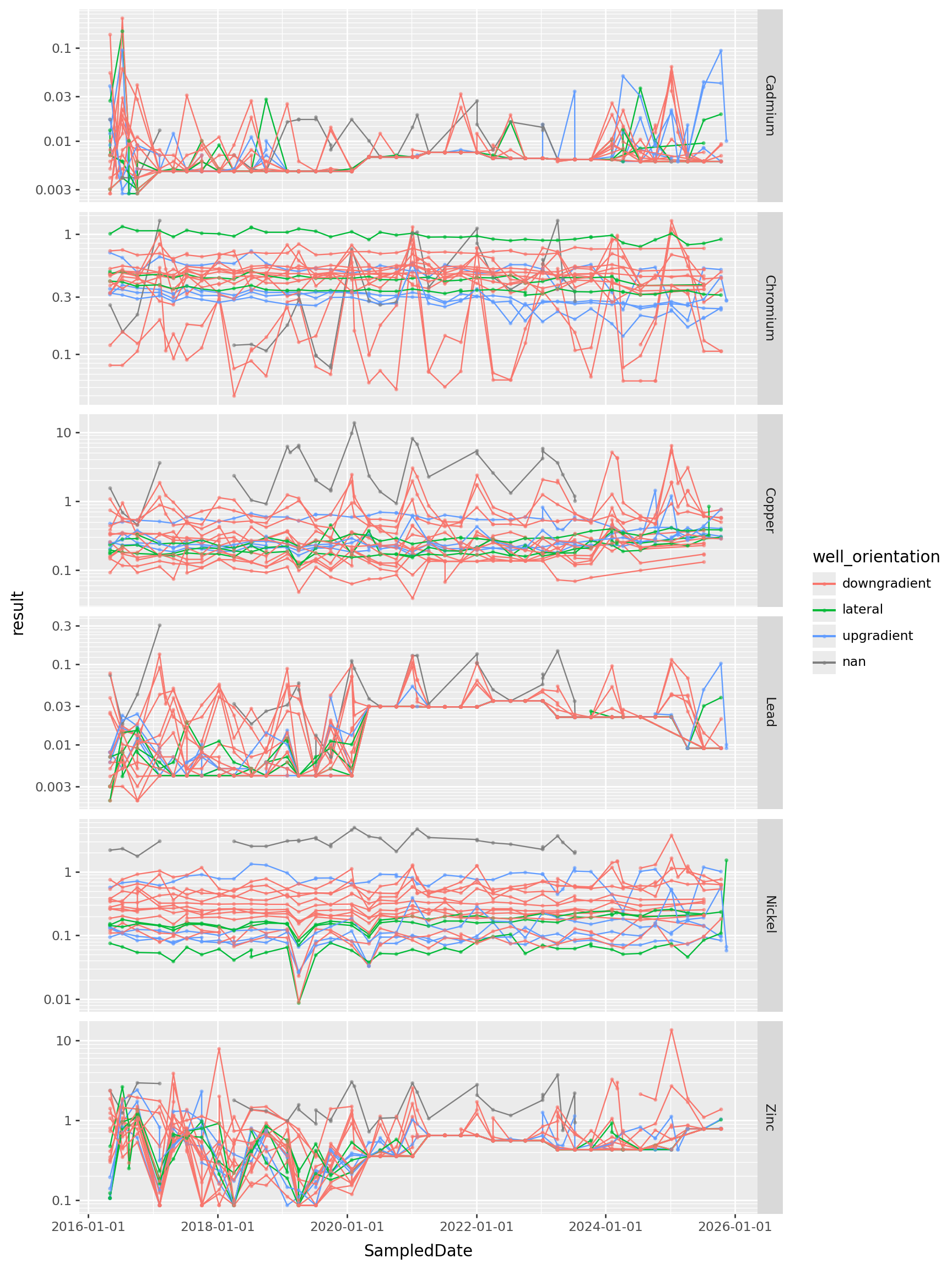

Takeaways?

Periodicity in water table elevation

Is the water table changing with the seasons? Looks like yes, although when it starts to come up again in the Fall seems to differ by year.

(
    gw
    .query("ParameterName == 'WaterTableElevation' and well_name == 'MW-17-1988'")
    >>
    p9.ggplot(p9.aes(x="SampledDate.dt.dayofyear", y="result", color='factor(SampledDate.dt.year)'))
    + p9.geom_point(size=0.5, alpha=0.75) + p9.geom_line()
    + p9.facet_wrap("well_name")
    + p9.labs(x='day of the year', y='level (ft)')
) + p9.theme(figure_size=(9,4))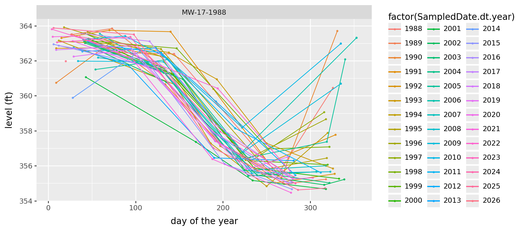

(
    gw
    .query("ParameterName == 'WaterTableElevation'")
    >>
    p9.ggplot(p9.aes(x="SampledDate.dt.dayofyear", y="result", color='factor(SampledDate.dt.year)'))
    + p9.geom_point(size=0.5, alpha=0.75) + p9.geom_line()
    + p9.facet_wrap("well_name")
    + p9.labs(x='day of the year', y='level (ft)')
) + p9.theme(figure_size=(9,15))

/home/peter/micromamba/envs/ds435/lib/python3.13/site-packages/plotnine/layer.py:374: PlotnineWarning: geom_point : Removed 7 rows containing missing values.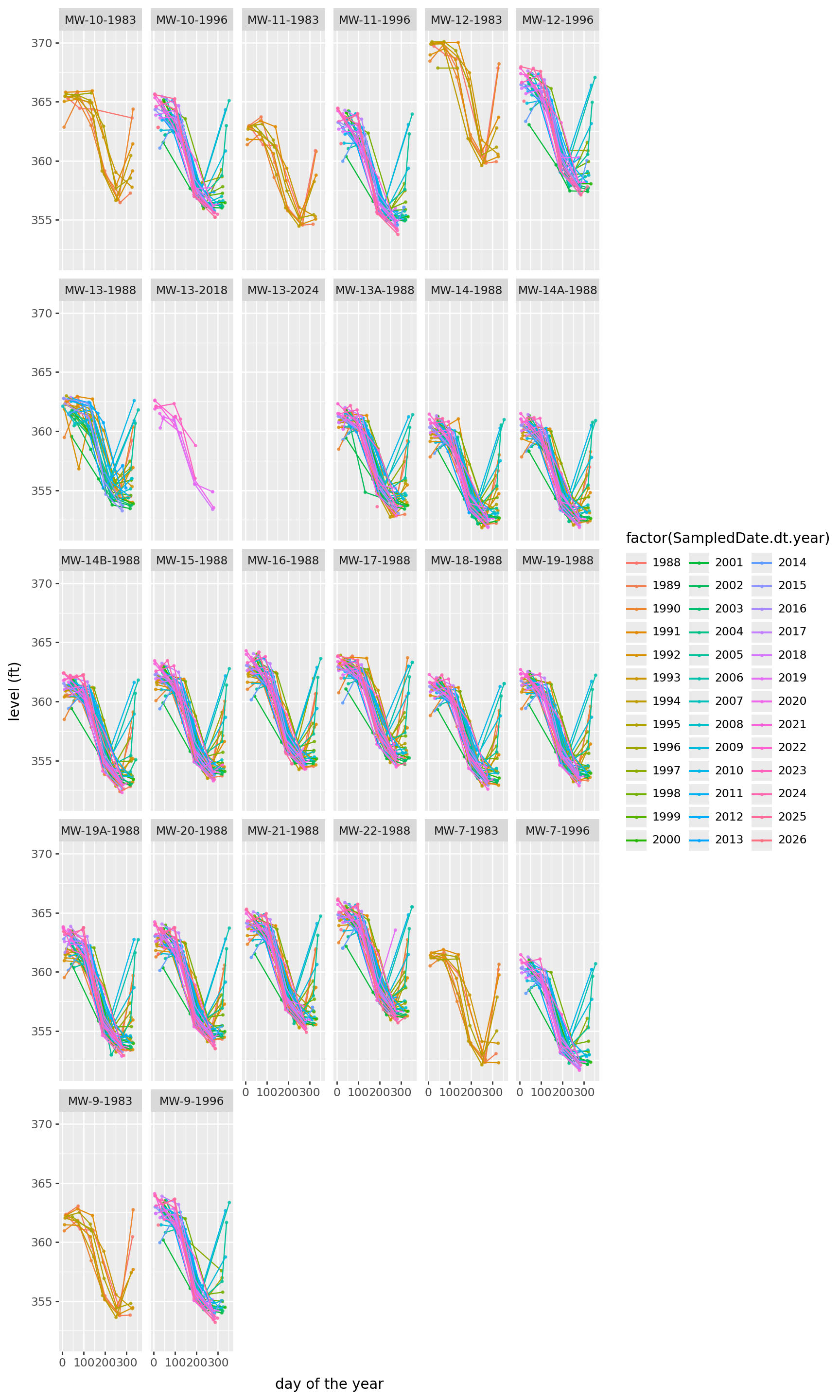

Conductivity

Let’s dive into conductivity:

Does the:

location relative to the plant,
or type of well

impact whether it’s:

increasing/decreasing long term,
or oscilating.

(
    gw.query("ParameterName == 'Conductivity'")
    >>
    p9.ggplot(p9.aes(x="SampledDate", y="result", color='well_depth_category', group='well_name'))
    + p9.geom_point(size=0.5, alpha=0.5) + p9.geom_line()
    + p9.labs(x='', y='conductivity (µS/cm)', title='Conductivity')
) + p9.theme(figure_size=(9,4))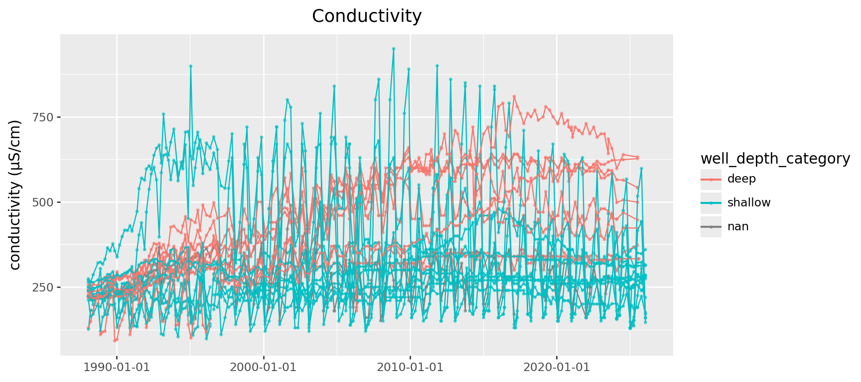

First step: separate out remove seasonal variation.

Model:

 value = seasonal + trend

conductivity = (
    gw
    .query("ParameterName == 'Conductivity'")
    .assign(year = lambda df: df['SampledDate'].dt.year)
    .assign(mean_conductivity = lambda df: df.groupby(['well_name', 'year'])['result'].transform("mean"))
    .assign(diff_conductivity = lambda df: df['result'] - df['mean_conductivity'])
)

(
    conductivity
    >>
    p9.ggplot(p9.aes(x="SampledDate", y="mean_conductivity", color='well_depth_category', group='well_name'))
    + p9.geom_point(size=0.2, alpha=0.25) + p9.geom_line()
    + p9.labs(x='', y='yearly mean', title='Conductivity (µS/cm)')
) / (
    conductivity
    >>
    p9.ggplot(p9.aes(x="SampledDate", y="diff_conductivity", color='well_depth_category', group='well_name'))
    + p9.geom_point(size=0.2, alpha=0.25) + p9.geom_line()
    + p9.labs(x='', y='seasonal difference')
) + p9.theme(figure_size=(9,6))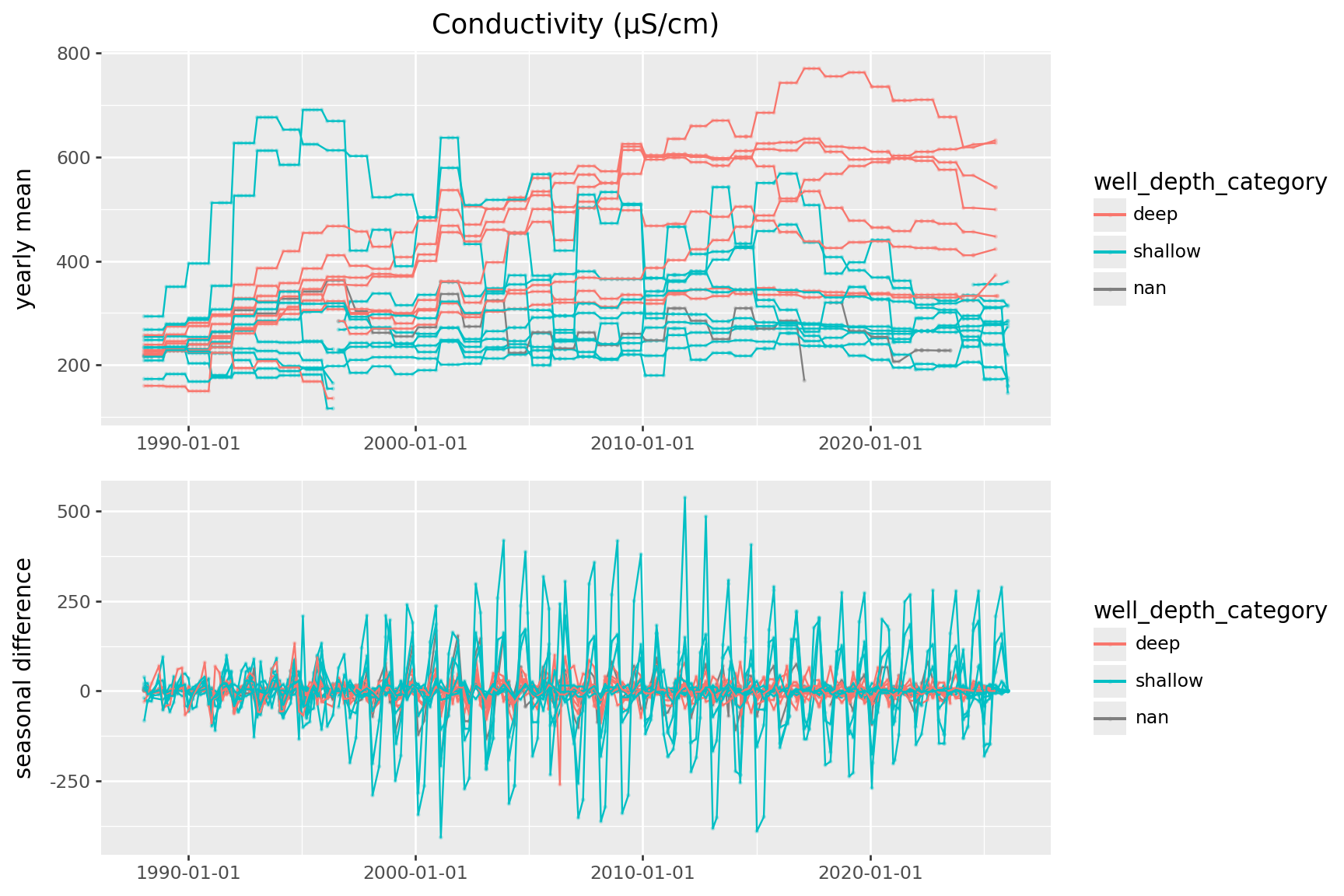

Per-well variability

The most variable wells are shallow:

csd = conductivity.groupby("well_name")['diff_conductivity'].std()
pd.merge(wells, pd.DataFrame(csd), on='well_name')[['well_name', 'diff_conductivity', 'well_orientation', 'well_depth_category']].sort_values("diff_conductivity")

	well_name	diff_conductivity	well_orientation	well_depth_category
3	MW-11-1996	6.911335	upgradient	shallow
15	MW-17-1988	7.788582	lateral	shallow
8	MW-13-2024	9.622023	downgradient	shallow
14	MW-16-1988	10.236792	lateral	deep
20	MW-21-1988	11.955536	lateral	shallow
23	MW-7-1996	12.942143	downgradient	deep
1	MW-10-1996	13.141271	upgradient	shallow
21	MW-22-1988	14.239555	upgradient	shallow
5	MW-12-1996	15.75467	upgradient	shallow
10	MW-14-1988	18.268072	downgradient	deep
25	MW-9-1996	19.788127	downgradient	shallow
2	MW-11-1983	21.207146	upgradient	shallow
11	MW-14A-1988	23.100607	downgradient	deep
16	MW-18-1988	24.80784	downgradient	deep
9	MW-13A-1988	25.516837	downgradient	deep
24	MW-9-1983	28.422397	downgradient	shallow
17	MW-19-1988	31.878937	downgradient	deep
13	MW-15-1988	36.719639	downgradient	deep
0	MW-10-1983	39.299083	upgradient	shallow
7	MW-13-2018	44.224813	<NA>	<NA>
22	MW-7-1983	51.630195	downgradient	deep
4	MW-12-1983	53.29468	upgradient	shallow
6	MW-13-1988	56.293998	<NA>	<NA>
18	MW-19A-1988	76.825087	downgradient	shallow
19	MW-20-1988	109.612696	downgradient	shallow
12	MW-14B-1988	201.358006	downgradient	shallow

Where are they?

And, mostly downgradient?

csdmap = make_colormap(csd.transform(np.log))
max_csd = csd.max()
legend_colors = { str(x) : csdmap(np.log(x)) for x in [1, int(max_csd/4), int(max_csd/2), int(max_csd*3/4), int(max_csd)] }

m = folium.Map(location=center, zoom_start=16)
for r in wells.itertuples():
    add_marker(
        m, r,
        fill_color=csdmap(np.log(csd[r.well_name])),
    )

add_legend(m, legend_colors, title='seasonality')
m

Make this Notebook Trusted to load map: File -> Trust Notebook

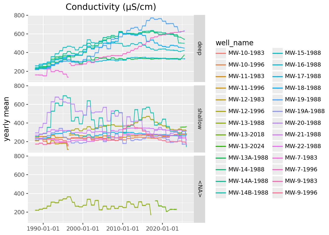
Long-term trends:

Looks like the big increases in conductivity are all at deep wells.

(
    conductivity
    >>
    p9.ggplot(p9.aes(x="SampledDate", y="mean_conductivity", color='well_name'))
    + p9.geom_point(size=0.2, alpha=0.25) + p9.geom_line()
    + p9.labs(x='', y='yearly mean', title='Conductivity (µS/cm)')
    + p9.facet_grid("well_depth_category")
)

Takeaways?

What’s correlated with what?

Question: what is “what”?

Refined question: which variables are correlated with each other, possibly considering seasonal variation or not?

Take 1: Per-observation correlation

wide_gw = (
    gw
    .set_index(['well_name', 'SampledDate', 'SampleNumber'])
    .loc[:,('ParameterName', 'ParameterUnits', 'result')]
    .pivot(columns='ParameterName', values='result')
    .reset_index()  
)
wide_gw.head()

ParameterName	well_name	SampledDate	SampleNumber	Ammonia	Cadmium	ChemicalOxygenDemand	Chloride	Chromium	Conductivity	Copper	...	Lead	Nickel	Nitrate	Temperature	TotalColiform	TotalDissolvedSolids	TotalOrganicCarbon	WaterTableElevation	Zinc	pH
0	MW-10-1983	1988-01-27	880068	0.1	1.0	5.0	1.9	5.0	238.0	5.0	...	5.0	5.0	3.8	<NA>	1.0	181.0	2.0	365.28	10.0	<NA>
1	MW-10-1983	1988-03-21	880248	0.1	1.0	10.0	4.5	5.0	238.0	5.0	...	5.0	5.0	6.0	<NA>	1.0	196.0	2.0	364.44	10.0	<NA>
2	MW-10-1983	1988-05-23	880426	0.1	1.0	10.0	3.1	5.0	198.0	5.0	...	5.0	10.0	4.7	<NA>	9.0	151.0	2.0	364.38	10.0	<NA>
3	MW-10-1983	1988-11-21	881128	0.1	1.0	10.0	2.8	5.0	192.0	15.0	...	5.0	10.0	4.9	<NA>	70.0	164.0	<NA>	363.63	10.0	<NA>
4	MW-10-1983	1989-01-26	890116	0.1	1.0	16.0	2.9	5.0	215.0	5.0	...	5.0	5.0	4.0	<NA>	1.0	169.0	<NA>	365.3	10.0	<NA>

5 rows × 21 columns

Take 1: The correlation matrix

cormat = wide_gw.select_dtypes("float").corr()
cormat.style.background_gradient()

ParameterName	Ammonia	Cadmium	ChemicalOxygenDemand	Chloride	Chromium	Conductivity	Copper	FecalColiform	Lead	Nickel	Nitrate	Temperature	TotalColiform	TotalDissolvedSolids	TotalOrganicCarbon	WaterTableElevation	Zinc	pH
ParameterName
Ammonia	1.000000	-0.071792	0.160236	0.037876	-0.074922	0.040336	-0.099566	-0.011911	-0.081283	-0.089971	0.019547	-0.093406	0.029169	0.026352	0.034601	-0.028478	-0.101453	-0.131407
Cadmium	-0.071792	1.000000	0.281764	-0.191022	0.863019	-0.307538	0.710645	0.038601	0.960762	0.913679	-0.084142	-0.129080	0.096055	-0.249209	0.507879	0.034189	0.749544	0.256278
ChemicalOxygenDemand	0.160236	0.281764	1.000000	-0.115090	0.286894	-0.158458	0.447788	0.076077	0.331570	0.373111	-0.146574	-0.142123	0.060277	-0.157341	0.342511	-0.000919	0.406129	0.038638
Chloride	0.037876	-0.191022	-0.115090	1.000000	-0.161892	0.469068	-0.207164	-0.057571	-0.204211	-0.186110	0.285950	0.295613	-0.048497	0.484853	-0.211492	-0.043363	-0.195340	0.017063
Chromium	-0.074922	0.863019	0.286894	-0.161892	1.000000	-0.259647	0.686521	0.032522	0.877213	0.839270	-0.065953	-0.133787	0.084074	-0.205510	0.444899	0.014855	0.727691	0.391783
Conductivity	0.040336	-0.307538	-0.158458	0.469068	-0.259647	1.000000	-0.310711	-0.088351	-0.315467	-0.281287	0.192999	0.372243	-0.086641	0.964487	-0.292122	-0.329148	-0.276213	0.164740
Copper	-0.099566	0.710645	0.447788	-0.207164	0.686521	-0.310711	1.000000	0.079348	0.800688	0.827862	-0.216518	-0.249487	0.130510	-0.263933	0.492412	0.000145	0.886070	0.090665
FecalColiform	-0.011911	0.038601	0.076077	-0.057571	0.032522	-0.088351	0.079348	1.000000	0.049238	0.052259	-0.050063	-0.057543	0.574707	-0.086840	0.211171	0.028351	0.040449	-0.147483
Lead	-0.081283	0.960762	0.331570	-0.204211	0.877213	-0.315467	0.800688	0.049238	1.000000	0.956844	-0.117430	-0.114198	0.099597	-0.257265	0.505792	0.016446	0.850833	0.269656
Nickel	-0.089971	0.913679	0.373111	-0.186110	0.839270	-0.281287	0.827862	0.052259	0.956844	1.000000	-0.165641	-0.194614	0.099505	-0.228114	0.526614	-0.014386	0.866621	0.162394
Nitrate	0.019547	-0.084142	-0.146574	0.285950	-0.065953	0.192999	-0.216518	-0.050063	-0.117430	-0.165641	1.000000	0.211520	-0.036594	0.257750	-0.234865	-0.049981	-0.187701	0.201779
Temperature	-0.093406	-0.129080	-0.142123	0.295613	-0.133787	0.372243	-0.249487	-0.057543	-0.114198	-0.194614	0.211520	1.000000	-0.216970	0.308916	-0.324921	-0.562670	-0.131932	0.459840
TotalColiform	0.029169	0.096055	0.060277	-0.048497	0.084074	-0.086641	0.130510	0.574707	0.099597	0.099505	-0.036594	-0.216970	1.000000	-0.087212	0.141671	0.017775	0.077223	-0.146319
TotalDissolvedSolids	0.026352	-0.249209	-0.157341	0.484853	-0.205510	0.964487	-0.263933	-0.086840	-0.257265	-0.228114	0.257750	0.308916	-0.087212	1.000000	-0.275284	-0.325074	-0.225765	0.156180
TotalOrganicCarbon	0.034601	0.507879	0.342511	-0.211492	0.444899	-0.292122	0.492412	0.211171	0.505792	0.526614	-0.234865	-0.324921	0.141671	-0.275284	1.000000	0.063420	0.413437	-0.406515
WaterTableElevation	-0.028478	0.034189	-0.000919	-0.043363	0.014855	-0.329148	0.000145	0.028351	0.016446	-0.014386	-0.049981	-0.562670	0.017775	-0.325074	0.063420	1.000000	-0.022563	-0.112165
Zinc	-0.101453	0.749544	0.406129	-0.195340	0.727691	-0.276213	0.886070	0.040449	0.850833	0.866621	-0.187701	-0.131932	0.077223	-0.225765	0.413437	-0.022563	1.000000	0.262602
pH	-0.131407	0.256278	0.038638	0.017063	0.391783	0.164740	0.090665	-0.147483	0.269656	0.162394	0.201779	0.459840	-0.146319	0.156180	-0.406515	-0.112165	0.262602	1.000000

Take 1: The correlation matrix, in a nice order:

cormat = wide_gw.select_dtypes("float").corr()
pcs = np.linalg.eig(cormat)
vord = np.argsort(np.abs(pcs.eigenvectors[:,0]))[::-1]

cormat.iloc[vord,vord].style.background_gradient()

ParameterName	Lead	Nickel	Cadmium	Zinc	Copper	Chromium	TotalOrganicCarbon	Conductivity	ChemicalOxygenDemand	TotalDissolvedSolids	Chloride	Temperature	Nitrate	TotalColiform	FecalColiform	pH	WaterTableElevation	Ammonia
ParameterName
Lead	1.000000	0.956844	0.960762	0.850833	0.800688	0.877213	0.505792	-0.315467	0.331570	-0.257265	-0.204211	-0.114198	-0.117430	0.099597	0.049238	0.269656	0.016446	-0.081283
Nickel	0.956844	1.000000	0.913679	0.866621	0.827862	0.839270	0.526614	-0.281287	0.373111	-0.228114	-0.186110	-0.194614	-0.165641	0.099505	0.052259	0.162394	-0.014386	-0.089971
Cadmium	0.960762	0.913679	1.000000	0.749544	0.710645	0.863019	0.507879	-0.307538	0.281764	-0.249209	-0.191022	-0.129080	-0.084142	0.096055	0.038601	0.256278	0.034189	-0.071792
Zinc	0.850833	0.866621	0.749544	1.000000	0.886070	0.727691	0.413437	-0.276213	0.406129	-0.225765	-0.195340	-0.131932	-0.187701	0.077223	0.040449	0.262602	-0.022563	-0.101453
Copper	0.800688	0.827862	0.710645	0.886070	1.000000	0.686521	0.492412	-0.310711	0.447788	-0.263933	-0.207164	-0.249487	-0.216518	0.130510	0.079348	0.090665	0.000145	-0.099566
Chromium	0.877213	0.839270	0.863019	0.727691	0.686521	1.000000	0.444899	-0.259647	0.286894	-0.205510	-0.161892	-0.133787	-0.065953	0.084074	0.032522	0.391783	0.014855	-0.074922
TotalOrganicCarbon	0.505792	0.526614	0.507879	0.413437	0.492412	0.444899	1.000000	-0.292122	0.342511	-0.275284	-0.211492	-0.324921	-0.234865	0.141671	0.211171	-0.406515	0.063420	0.034601
Conductivity	-0.315467	-0.281287	-0.307538	-0.276213	-0.310711	-0.259647	-0.292122	1.000000	-0.158458	0.964487	0.469068	0.372243	0.192999	-0.086641	-0.088351	0.164740	-0.329148	0.040336
ChemicalOxygenDemand	0.331570	0.373111	0.281764	0.406129	0.447788	0.286894	0.342511	-0.158458	1.000000	-0.157341	-0.115090	-0.142123	-0.146574	0.060277	0.076077	0.038638	-0.000919	0.160236
TotalDissolvedSolids	-0.257265	-0.228114	-0.249209	-0.225765	-0.263933	-0.205510	-0.275284	0.964487	-0.157341	1.000000	0.484853	0.308916	0.257750	-0.087212	-0.086840	0.156180	-0.325074	0.026352
Chloride	-0.204211	-0.186110	-0.191022	-0.195340	-0.207164	-0.161892	-0.211492	0.469068	-0.115090	0.484853	1.000000	0.295613	0.285950	-0.048497	-0.057571	0.017063	-0.043363	0.037876
Temperature	-0.114198	-0.194614	-0.129080	-0.131932	-0.249487	-0.133787	-0.324921	0.372243	-0.142123	0.308916	0.295613	1.000000	0.211520	-0.216970	-0.057543	0.459840	-0.562670	-0.093406
Nitrate	-0.117430	-0.165641	-0.084142	-0.187701	-0.216518	-0.065953	-0.234865	0.192999	-0.146574	0.257750	0.285950	0.211520	1.000000	-0.036594	-0.050063	0.201779	-0.049981	0.019547
TotalColiform	0.099597	0.099505	0.096055	0.077223	0.130510	0.084074	0.141671	-0.086641	0.060277	-0.087212	-0.048497	-0.216970	-0.036594	1.000000	0.574707	-0.146319	0.017775	0.029169
FecalColiform	0.049238	0.052259	0.038601	0.040449	0.079348	0.032522	0.211171	-0.088351	0.076077	-0.086840	-0.057571	-0.057543	-0.050063	0.574707	1.000000	-0.147483	0.028351	-0.011911
pH	0.269656	0.162394	0.256278	0.262602	0.090665	0.391783	-0.406515	0.164740	0.038638	0.156180	0.017063	0.459840	0.201779	-0.146319	-0.147483	1.000000	-0.112165	-0.131407
WaterTableElevation	0.016446	-0.014386	0.034189	-0.022563	0.000145	0.014855	0.063420	-0.329148	-0.000919	-0.325074	-0.043363	-0.562670	-0.049981	0.017775	0.028351	-0.112165	1.000000	-0.028478
Ammonia	-0.081283	-0.089971	-0.071792	-0.101453	-0.099566	-0.074922	0.034601	0.040336	0.160236	0.026352	0.037876	-0.093406	0.019547	0.029169	-0.011911	-0.131407	-0.028478	1.000000

Take 2: Per-year (average) correlation:

yearly_gw = (
    gw
    .assign(year = lambda df: df['SampledDate'].dt.year)
    .set_index(['well_name', 'ParameterName'])
    .select_dtypes(("number", "datetime"))
    .groupby(['well_name', 'year', 'ParameterName'])
    .mean()
    .reset_index()
    .set_index(['well_name', 'SampledDate'])
    .loc[:,('ParameterName', 'result')]
    .pivot(columns='ParameterName', values='result')
    .reset_index()
)
yearly_gw.head()

ParameterName	well_name	SampledDate	Ammonia	Cadmium	ChemicalOxygenDemand	Chloride	Chromium	Conductivity	Copper	FecalColiform	Lead	Nickel	Nitrate	Temperature	TotalColiform	TotalDissolvedSolids	TotalOrganicCarbon	WaterTableElevation	Zinc	pH
0	MW-10-1983	1988-03-24 00:00:00	<NA>	<NA>	<NA>	<NA>	<NA>	<NA>	<NA>	<NA>	<NA>	<NA>	<NA>	<NA>	<NA>	<NA>	2.0	<NA>	<NA>	<NA>
1	MW-10-1983	1988-05-23 12:00:00	0.1	1.0	8.75	3.075	5.0	216.5	7.5	10.75	5.0	7.5	4.85	<NA>	20.25	173.0	<NA>	364.4325	10.0	<NA>
2	MW-10-1983	1989-05-29 19:12:00	<NA>	<NA>	<NA>	<NA>	<NA>	<NA>	<NA>	<NA>	<NA>	<NA>	<NA>	<NA>	201.0	<NA>	<NA>	<NA>	<NA>	<NA>
3	MW-10-1983	1989-06-18 20:00:00	0.1	1.0	11.0	2.183333	5.0	227.5	5.0	35.0	5.0	7.5	2.816667	<NA>	<NA>	171.5	<NA>	361.25	10.0	<NA>
4	MW-10-1983	1989-07-17 14:24:00	<NA>	<NA>	<NA>	<NA>	<NA>	<NA>	<NA>	<NA>	<NA>	<NA>	<NA>	<NA>	<NA>	<NA>	3.0	<NA>	<NA>	<NA>

Take 2: correlation matrix

Cor(temperature, ammonia) is NA, so we omit it:

cormat = yearly_gw.drop(columns="Temperature").select_dtypes("float").corr()
pcs = np.linalg.eig(cormat)
vord = np.argsort(np.abs(pcs.eigenvectors[:,0]))[::-1]
cormat.iloc[vord,vord].style.background_gradient()

ParameterName	Nickel	Lead	Copper	Cadmium	Zinc	Chromium	Conductivity	TotalOrganicCarbon	TotalDissolvedSolids	ChemicalOxygenDemand	Chloride	pH	Nitrate	TotalColiform	FecalColiform	WaterTableElevation	Ammonia
ParameterName
Nickel	1.000000	0.974307	0.873757	0.914269	0.839927	0.932369	-0.443580	0.519879	-0.329528	0.382999	-0.258540	-0.606327	-0.262817	0.152710	0.113619	0.113584	-0.111252
Lead	0.974307	1.000000	0.822724	0.963876	0.793517	0.962665	-0.465164	0.459696	-0.339230	0.329172	-0.278216	-0.354037	-0.218795	0.153477	0.132039	0.102502	-0.082002
Copper	0.873757	0.822724	1.000000	0.659877	0.947138	0.731038	-0.486004	0.407220	-0.390038	0.458215	-0.293347	-0.608708	-0.268430	0.185043	0.146225	0.133345	-0.145061
Cadmium	0.914269	0.963876	0.659877	1.000000	0.634862	0.960553	-0.463534	0.466456	-0.331818	0.237424	-0.268653	-0.177833	-0.208729	0.149995	0.126472	0.099417	-0.108828
Zinc	0.839927	0.793517	0.947138	0.634862	1.000000	0.707477	-0.485474	0.366917	-0.357321	0.440482	-0.285125	-0.351361	-0.246009	0.152437	0.133209	0.111473	-0.105533
Chromium	0.932369	0.962665	0.731038	0.960553	0.707477	1.000000	-0.448873	0.453482	-0.329363	0.288018	-0.266127	0.334352	-0.184797	0.143222	0.119331	0.083056	-0.106301
Conductivity	-0.443580	-0.465164	-0.486004	-0.463534	-0.485474	-0.448873	1.000000	-0.381327	0.983868	-0.417007	0.493450	0.095067	0.173398	-0.149138	-0.142508	-0.406708	-0.024878
TotalOrganicCarbon	0.519879	0.459696	0.407220	0.466456	0.366917	0.453482	-0.381327	1.000000	-0.317408	0.361808	-0.293275	-0.498195	-0.431739	0.215832	0.251730	0.168075	0.003362
TotalDissolvedSolids	-0.329528	-0.339230	-0.390038	-0.331818	-0.357321	-0.329363	0.983868	-0.317408	1.000000	-0.314850	0.450307	0.019255	0.251597	-0.149055	-0.148365	-0.419909	-0.007653
ChemicalOxygenDemand	0.382999	0.329172	0.458215	0.237424	0.440482	0.288018	-0.417007	0.361808	-0.314850	1.000000	-0.254168	-0.199517	-0.280234	0.120198	0.121035	0.170892	0.376442
Chloride	-0.258540	-0.278216	-0.293347	-0.268653	-0.285125	-0.266127	0.493450	-0.293275	0.450307	-0.254168	1.000000	-0.064295	0.274520	-0.065459	-0.082674	0.005607	0.029020
pH	-0.606327	-0.354037	-0.608708	-0.177833	-0.351361	0.334352	0.095067	-0.498195	0.019255	-0.199517	-0.064295	1.000000	0.199231	-0.263690	-0.222692	-0.038003	-0.036537
Nitrate	-0.262817	-0.218795	-0.268430	-0.208729	-0.246009	-0.184797	0.173398	-0.431739	0.251597	-0.280234	0.274520	0.199231	1.000000	-0.062496	-0.064400	-0.031481	0.035847
TotalColiform	0.152710	0.153477	0.185043	0.149995	0.152437	0.143222	-0.149138	0.215832	-0.149055	0.120198	-0.065459	-0.263690	-0.062496	1.000000	0.781211	0.111059	0.011857
FecalColiform	0.113619	0.132039	0.146225	0.126472	0.133209	0.119331	-0.142508	0.251730	-0.148365	0.121035	-0.082674	-0.222692	-0.064400	0.781211	1.000000	0.045777	-0.009722
WaterTableElevation	0.113584	0.102502	0.133345	0.099417	0.111473	0.083056	-0.406708	0.168075	-0.419909	0.170892	0.005607	-0.038003	-0.031481	0.111059	0.045777	1.000000	0.040060
Ammonia	-0.111252	-0.082002	-0.145061	-0.108828	-0.105533	-0.106301	-0.024878	0.003362	-0.007653	0.376442	0.029020	-0.036537	0.035847	0.011857	-0.009722	0.040060	1.000000

Take 3: Per-year averages, since 2016

recent_gw = (
    gw
    .query("SampledDate >= '01-01-2016'")
    .assign(year = lambda df: df['SampledDate'].dt.year)
    .set_index(['well_name', 'ParameterName'])
    .select_dtypes(("number", "datetime"))
    .groupby(['well_name', 'year', 'ParameterName'])
    .mean()
    .reset_index()
    .set_index(['well_name', 'SampledDate'])
    .loc[:,('ParameterName', 'result')]
    .pivot(columns='ParameterName', values='result')
    .reset_index()
)
recent_gw.head()

ParameterName	well_name	SampledDate	Ammonia	Cadmium	ChemicalOxygenDemand	Chloride	Chromium	Conductivity	Copper	FecalColiform	Lead	Nickel	Nitrate	Temperature	TotalColiform	TotalDissolvedSolids	TotalOrganicCarbon	WaterTableElevation	Zinc	pH
0	MW-10-1996	2016-05-31 00:00:00	0.1	<NA>	<NA>	3.55	<NA>	<NA>	<NA>	1.0	<NA>	<NA>	3.525	<NA>	1.0	170.0	<NA>	<NA>	<NA>	<NA>
1	MW-10-1996	2016-06-15 19:12:00	<NA>	<NA>	<NA>	<NA>	<NA>	240.0	<NA>	<NA>	<NA>	<NA>	<NA>	<NA>	<NA>	<NA>	<NA>	359.66	<NA>	7.02
2	MW-10-1996	2016-07-16 16:00:00	<NA>	<NA>	5.0	<NA>	0.35	<NA>	0.265	<NA>	0.011667	0.1	<NA>	<NA>	<NA>	<NA>	0.5	<NA>	0.9192	<NA>
3	MW-10-1996	2016-07-24 18:00:00	<NA>	0.028675	<NA>	<NA>	<NA>	<NA>	<NA>	<NA>	<NA>	<NA>	<NA>	<NA>	<NA>	<NA>	<NA>	<NA>	<NA>	<NA>
4	MW-10-1996	2017-06-18 00:00:00	0.1	0.005083	5.0	3.516667	0.338	236.666667	0.236667	1.0	0.005233	0.085	3.816667	<NA>	1.0	166.666667	0.816667	360.96	0.746317	6.966667

Take 3: correlation matrix

cormat = recent_gw.drop(columns="Temperature").select_dtypes("float").corr()
pcs = np.linalg.eig(cormat)
vord = np.argsort(np.abs(pcs.eigenvectors[:,0]))[::-1]
cormat.iloc[vord,vord].style.background_gradient()

ParameterName	TotalOrganicCarbon	Copper	Nickel	Lead	Zinc	pH	Conductivity	TotalDissolvedSolids	ChemicalOxygenDemand	Cadmium	TotalColiform	Nitrate	FecalColiform	WaterTableElevation	Chloride	Ammonia	Chromium
ParameterName
TotalOrganicCarbon	1.000000	0.890807	0.878169	0.753568	0.581503	-0.498195	-0.220552	-0.251105	0.573421	0.283312	0.241063	-0.378747	0.262582	0.216115	-0.222661	0.056656	0.130319
Copper	0.890807	1.000000	0.909084	0.610292	0.628322	-0.608708	-0.322752	-0.301071	0.352848	0.344804	0.310256	-0.275047	0.167236	0.162293	-0.073357	-0.060376	0.135102
Nickel	0.878169	0.909084	1.000000	0.562719	0.650353	-0.606327	-0.201874	-0.133684	0.311853	0.357334	0.215208	-0.262286	0.359429	0.155727	0.074074	-0.068902	0.055345
Lead	0.753568	0.610292	0.562719	1.000000	0.491133	-0.354037	-0.244525	-0.213029	0.597012	0.283380	0.204370	-0.205487	0.055351	0.257111	-0.170673	0.128016	0.244156
Zinc	0.581503	0.628322	0.650353	0.491133	1.000000	-0.351361	-0.268892	-0.204725	0.098982	0.432160	0.187908	-0.213891	0.188980	0.084388	-0.099996	-0.117539	0.094888
pH	-0.498195	-0.608708	-0.606327	-0.354037	-0.351361	1.000000	0.241367	0.190971	-0.199517	-0.177833	-0.393534	0.289830	-0.354504	-0.231699	0.007443	-0.031606	0.334352
Conductivity	-0.220552	-0.322752	-0.201874	-0.244525	-0.268892	0.241367	1.000000	0.984912	-0.186379	-0.163036	-0.123750	0.254431	-0.110083	-0.586880	0.369098	0.015135	0.125407
TotalDissolvedSolids	-0.251105	-0.301071	-0.133684	-0.213029	-0.204725	0.190971	0.984912	1.000000	-0.189485	-0.240204	-0.167343	0.325359	-0.151245	-0.622172	0.350088	-0.028149	0.171769
ChemicalOxygenDemand	0.573421	0.352848	0.311853	0.597012	0.098982	-0.199517	-0.186379	-0.189485	1.000000	0.119445	-0.007333	-0.196866	0.038757	0.224439	-0.138664	0.602247	0.089381
Cadmium	0.283312	0.344804	0.357334	0.283380	0.432160	-0.177833	-0.163036	-0.240204	0.119445	1.000000	0.244746	-0.124114	0.324230	0.097763	-0.202166	-0.066868	0.078485
TotalColiform	0.241063	0.310256	0.215208	0.204370	0.187908	-0.393534	-0.123750	-0.167343	-0.007333	0.244746	1.000000	-0.043623	0.983906	0.094847	-0.107008	-0.056771	-0.083557
Nitrate	-0.378747	-0.275047	-0.262286	-0.205487	-0.213891	0.289830	0.254431	0.325359	-0.196866	-0.124114	-0.043623	1.000000	-0.049502	-0.214486	0.279763	0.018544	0.489560
FecalColiform	0.262582	0.167236	0.359429	0.055351	0.188980	-0.354504	-0.110083	-0.151245	0.038757	0.324230	0.983906	-0.049502	1.000000	0.095345	-0.094697	-0.023470	-0.153142
WaterTableElevation	0.216115	0.162293	0.155727	0.257111	0.084388	-0.231699	-0.586880	-0.622172	0.224439	0.097763	0.094847	-0.214486	0.095345	1.000000	0.045799	-0.030745	-0.058456
Chloride	-0.222661	-0.073357	0.074074	-0.170673	-0.099996	0.007443	0.369098	0.350088	-0.138664	-0.202166	-0.107008	0.279763	-0.094697	0.045799	1.000000	-0.012760	0.137604
Ammonia	0.056656	-0.060376	-0.068902	0.128016	-0.117539	-0.031606	0.015135	-0.028149	0.602247	-0.066868	-0.056771	0.018544	-0.023470	-0.030745	-0.012760	1.000000	0.080543
Chromium	0.130319	0.135102	0.055345	0.244156	0.094888	0.334352	0.125407	0.171769	0.089381	0.078485	-0.083557	0.489560	-0.153142	-0.058456	0.137604	0.080543	1.000000

Takeaways:

Note: two variables are strongly correlated here if they tend to have larger-than-average values in the same year-well combinations.

So, this might be “the two variables are typically higher in the same wells”, or “the two variables are typically higher in the same years”, or some complicated combination.

“Look at the data”, part 3?

Next steps: brainstorm!

Ideas? Questions?

Do nearby wells get similar measurements?