Case study: Groundwater monitoring
2026-02-16
What is measured?
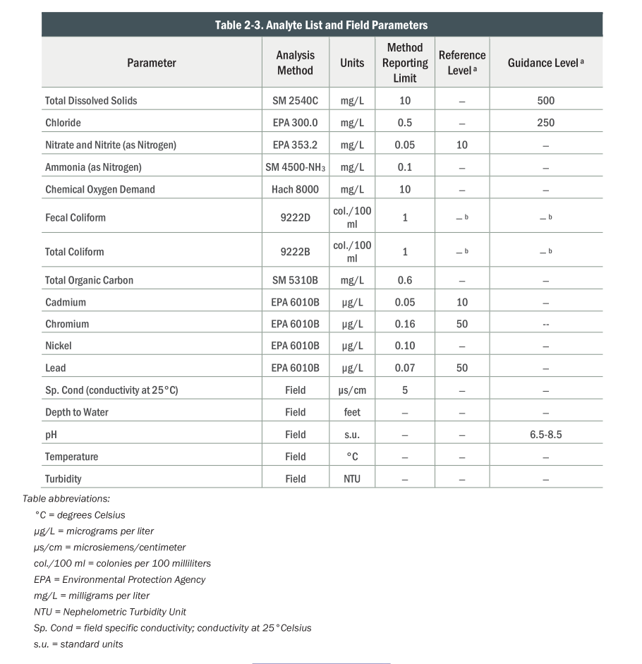 )
)
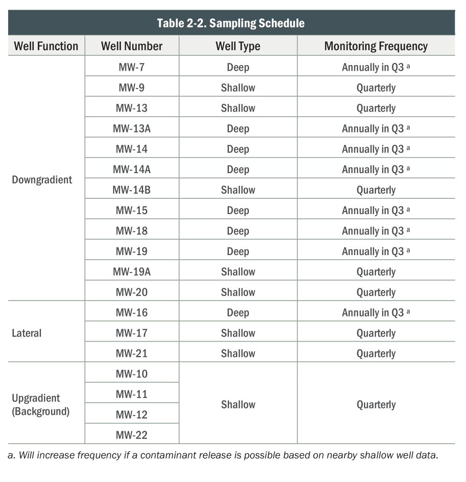
When was each well used?
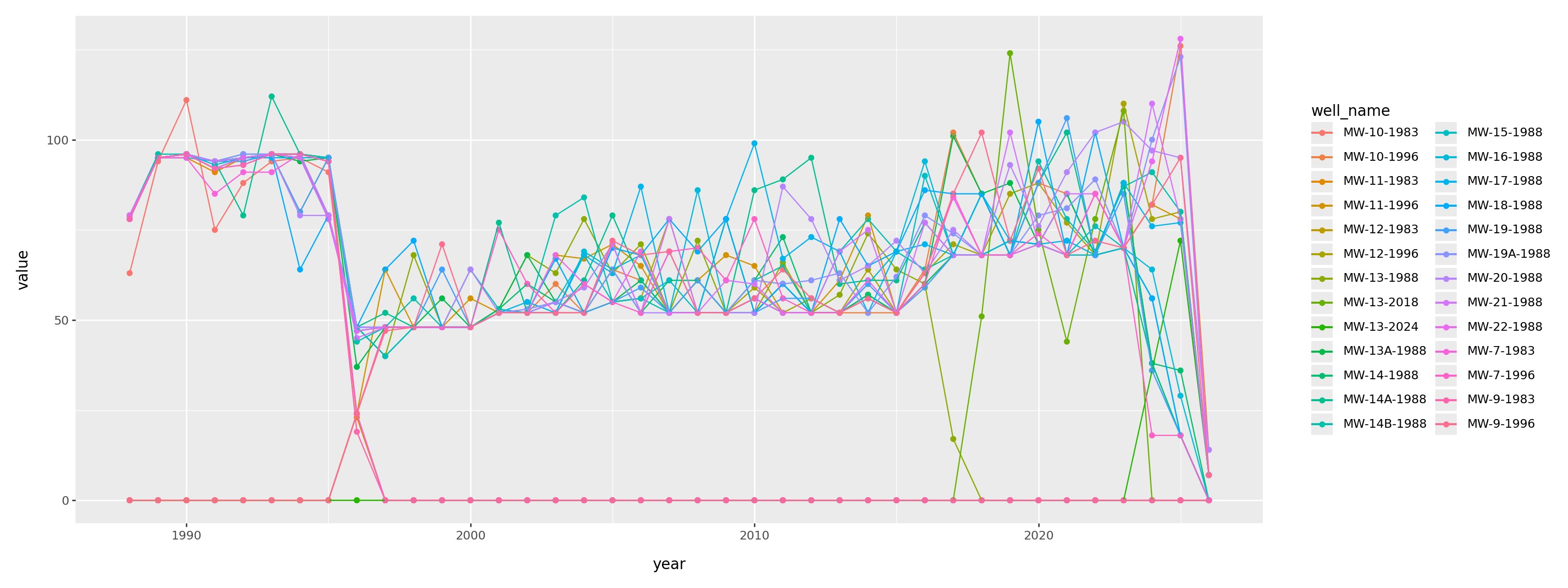
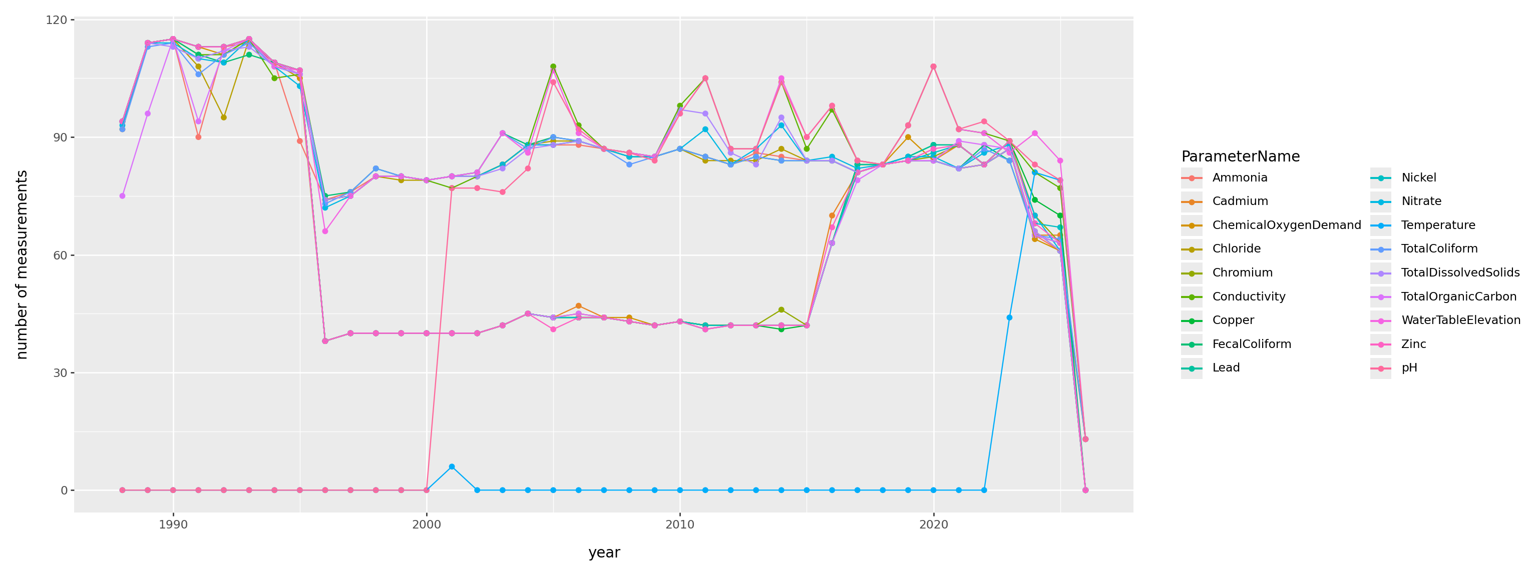
When was each thing measured?
(
    pd.crosstab(gw['ParameterName'], gw['SampledDate'].dt.year)
    .reset_index()
    .melt(id_vars=['ParameterName'])
    .assign(year=lambda df: pd.to_numeric(df['SampledDate']))
    >>
    p9.ggplot(p9.aes(x='year', y='value', color='ParameterName'))
    + p9.geom_point() + p9.geom_line()
    + p9.labs(y='number of measurements')
    + p9.theme(figure_size=(16,6))
)
All the data, from 20,000 feet
/home/peter/micromamba/envs/ds435/lib/python3.13/site-packages/plotnine/layer.py:374: PlotnineWarning: geom_point : Removed 7 rows containing missing values.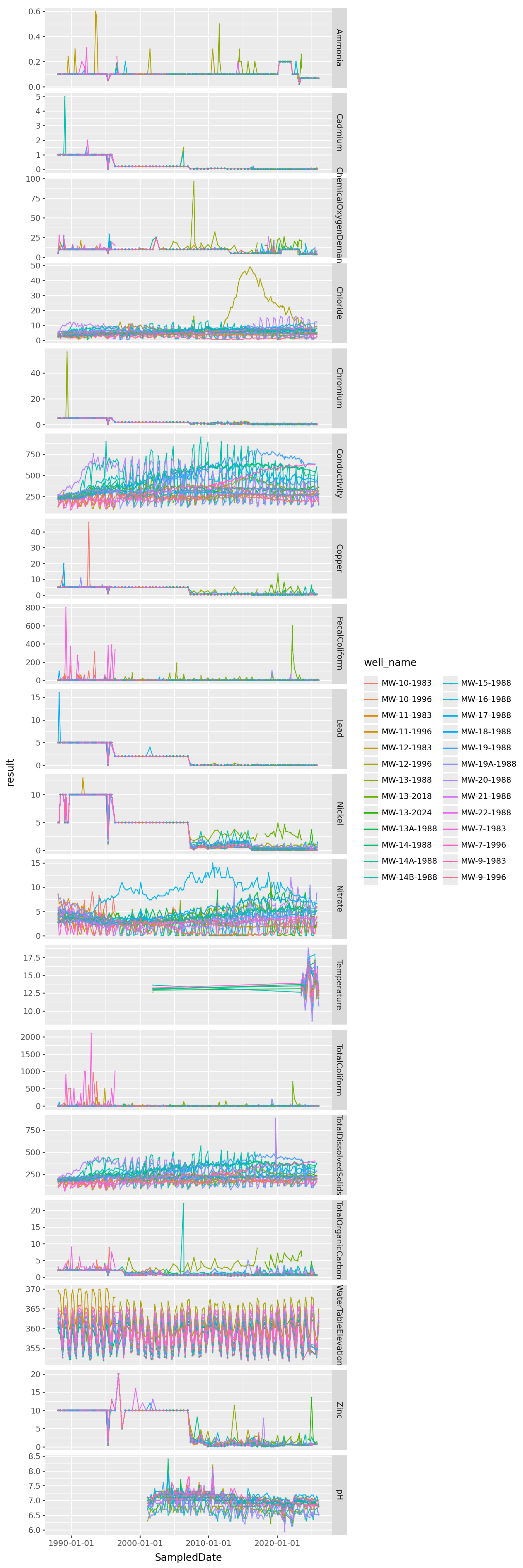
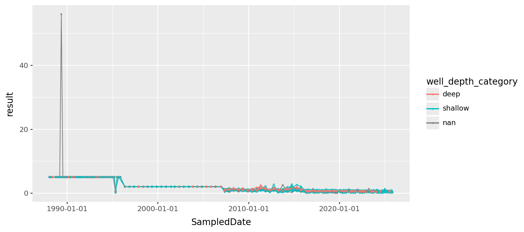
Here’s Chromium:
Chromium, transformed
(
    gw
    .query("ParameterName == 'Chromium'")
    >> p9.ggplot(p9.aes(x="SampledDate", y="result", color="well_depth_category", group="well_name"))
    + p9.geom_line() + p9.geom_point(size=0.5, alpha=0.5)
    + p9.labs(title="Chromium", y="concentration (µg/L)")
    + p9.scale_y_log10()
) + p9.theme(figure_size=(9,4))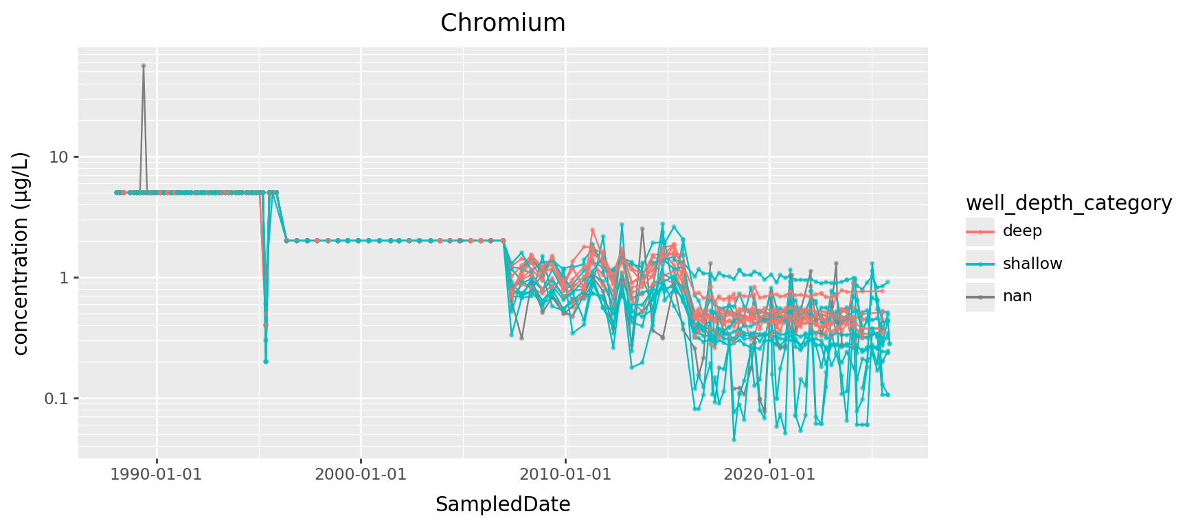
Chromium, “identifying outliers”?
z = (value - center) / scale
Question: what to use for “center” and “scale”? Median+IQR or mean+SD? Within groups? Which groups?
- Definitely group by year in this case, since things change.
- Usually I’d prefer “median and IQR”, but for many years the IQR is zero.
chromium = (
    gw.query("ParameterName == 'Chromium'")
    .assign(
        mean = lambda df: df['result'].groupby(df['SampledDate'].dt.year).transform('mean'),
        std = lambda df: df['result'].groupby(df['SampledDate'].dt.year).transform('std'),
        z = lambda df: (df['result'] - df['mean']) / ( df['std'] + (df['std'] == 0) ),
    )
)
chromium >> p9.ggplot(p9.aes(x='z')) + p9.geom_histogram(bins=40)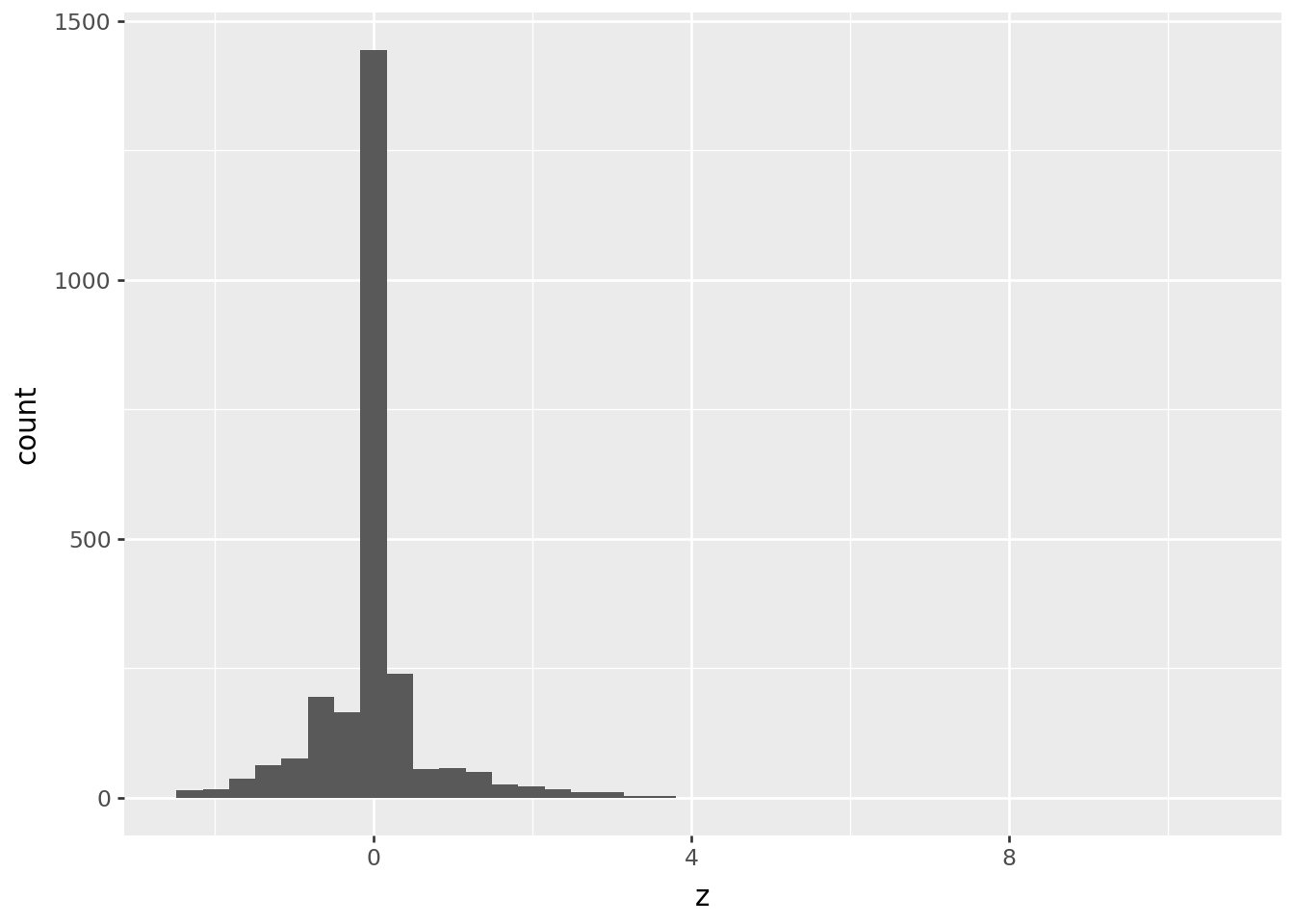
How’s that look?
The cutoff for “outlier” in terms of \(z\) scores should always be made looking at the data, but often between 3 and 5 is good, if this is a reasonable approach.
p1 = (
    chromium
    >>
    p9.ggplot(p9.aes(x="SampledDate", y="result", group="well_name"))
    + p9.geom_line(alpha=0.5)
    + p9.geom_point(mapping=p9.aes(color="z.abs() > 5"))
    + p9.labs(title="Chromium", y="concentration (µg/L)")
)
p2 = (
    chromium
    .query("abs(z) < 5")
    >>
    p9.ggplot(p9.aes(x="SampledDate", y="result", group="well_name"))
    + p9.geom_line(alpha=0.5)
    + p9.geom_point()
    + p9.labs(title="Chromium", y="concentration (µg/L)")
)
(p1 / p2)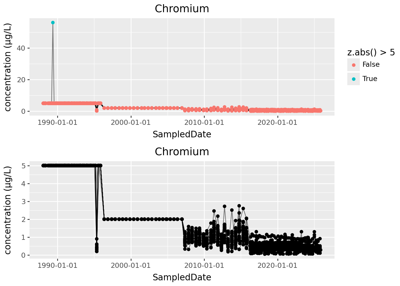
All the heavy metals
metals = ["Cadmium", "Chromium", "Copper", "Lead", "Nickel", "Zinc"]
(
    gw
    .loc[gw['ParameterName'].isin(metals), :]
    >> p9.ggplot(p9.aes(x="SampledDate", y="result", color="well_orientation", group="well_name"))
    + p9.geom_line() + p9.geom_point(size=0.5, alpha=0.5)
    + p9.scale_y_log10()
    + p9.facet_grid(rows="ParameterName")
) + p9.theme(figure_size=(9,12))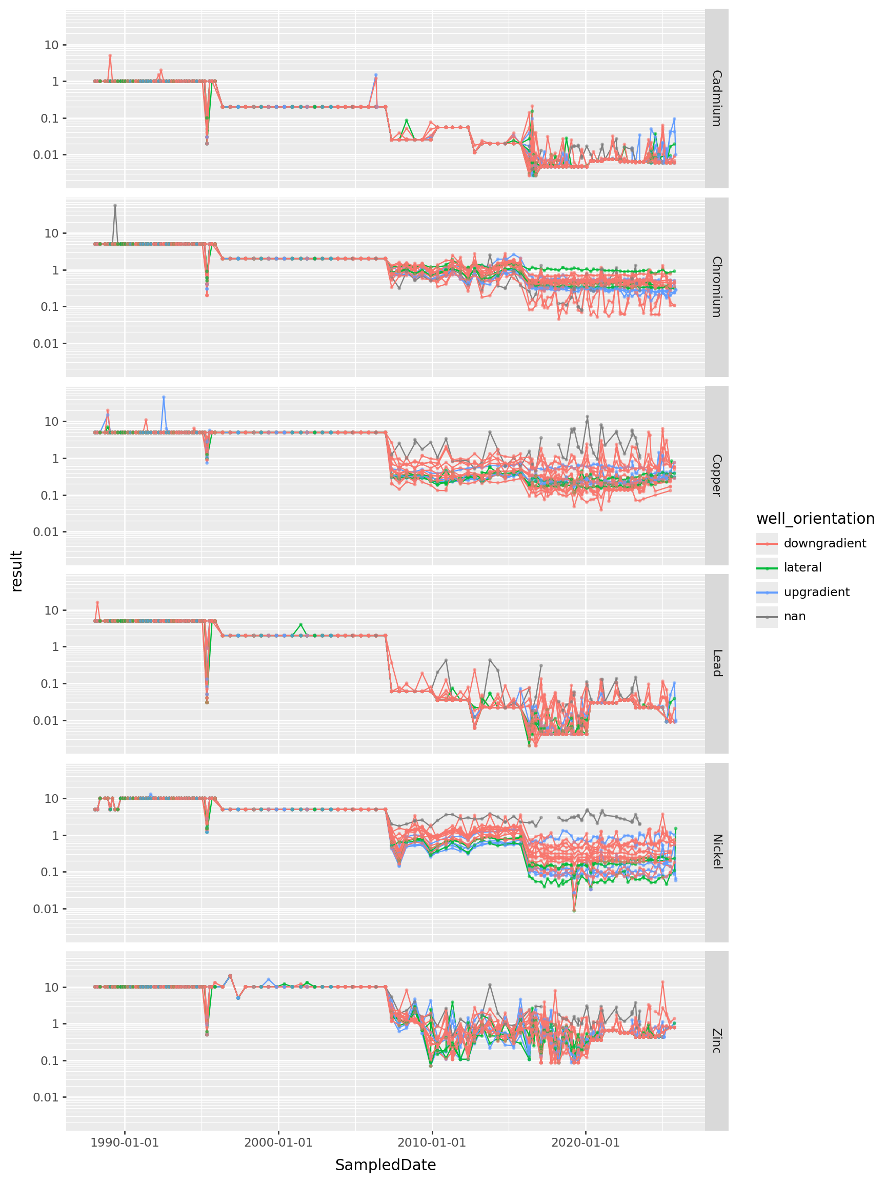
All the heavy metals, since 2016
(
    gw
    .loc[(gw['ParameterName'].isin(metals)) & (gw['SampledDate'].dt.year >= 2016), :]
    >> p9.ggplot(p9.aes(x="SampledDate", y="result", color="well_orientation", group="well_name"))
    + p9.geom_line() + p9.geom_point(size=0.5, alpha=0.5)
    + p9.scale_y_log10()
    + p9.facet_grid(rows="ParameterName", scales="free_y")
) + p9.theme(figure_size=(9,12))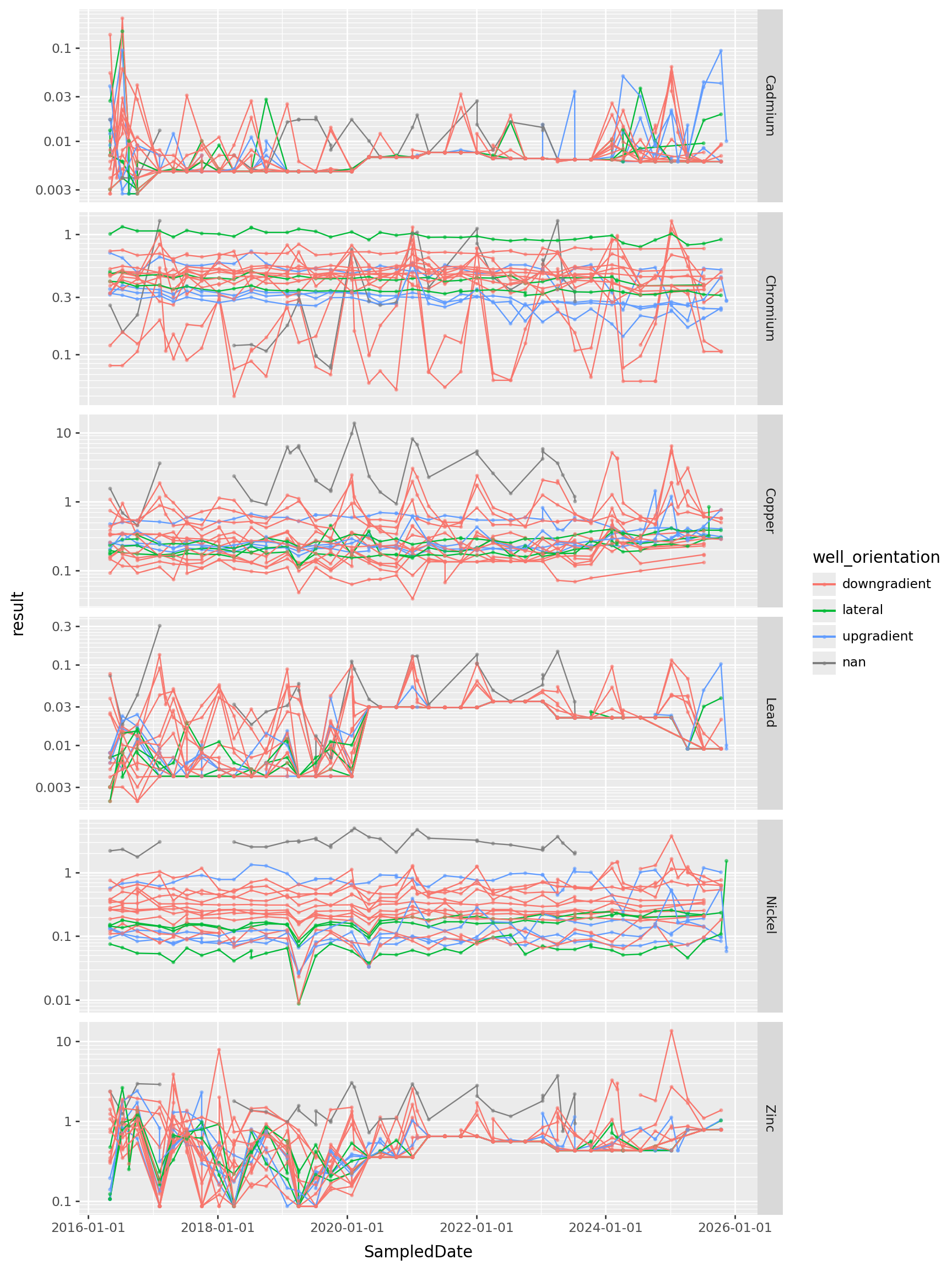
Periodicity in water table elevation
Is the water table changing with the seasons? Looks like yes, although when it starts to come up again in the Fall seems to differ by year.
(
    gw
    .query("ParameterName == 'WaterTableElevation' and well_name == 'MW-17-1988'")
    >>
    p9.ggplot(p9.aes(x="SampledDate.dt.dayofyear", y="result", color='factor(SampledDate.dt.year)'))
    + p9.geom_point(size=0.5, alpha=0.75) + p9.geom_line()
    + p9.facet_wrap("well_name")
    + p9.labs(x='day of the year', y='level (ft)')
) + p9.theme(figure_size=(9,4))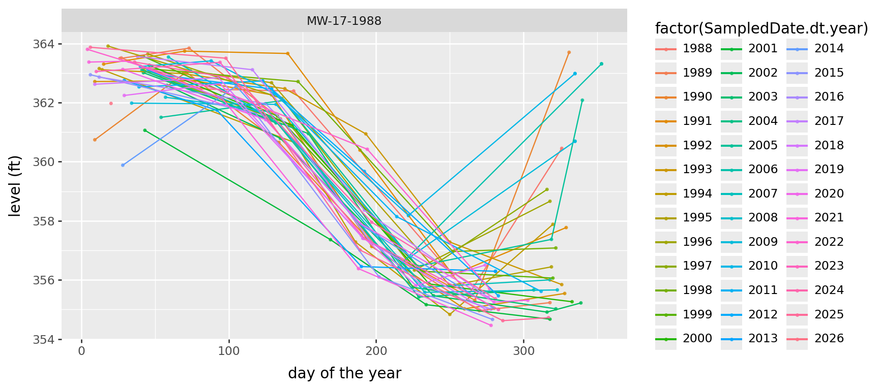
(
    gw
    .query("ParameterName == 'WaterTableElevation'")
    >>
    p9.ggplot(p9.aes(x="SampledDate.dt.dayofyear", y="result", color='factor(SampledDate.dt.year)'))
    + p9.geom_point(size=0.5, alpha=0.75) + p9.geom_line()
    + p9.facet_wrap("well_name")
    + p9.labs(x='day of the year', y='level (ft)')
) + p9.theme(figure_size=(9,15))
/home/peter/micromamba/envs/ds435/lib/python3.13/site-packages/plotnine/layer.py:374: PlotnineWarning: geom_point : Removed 7 rows containing missing values.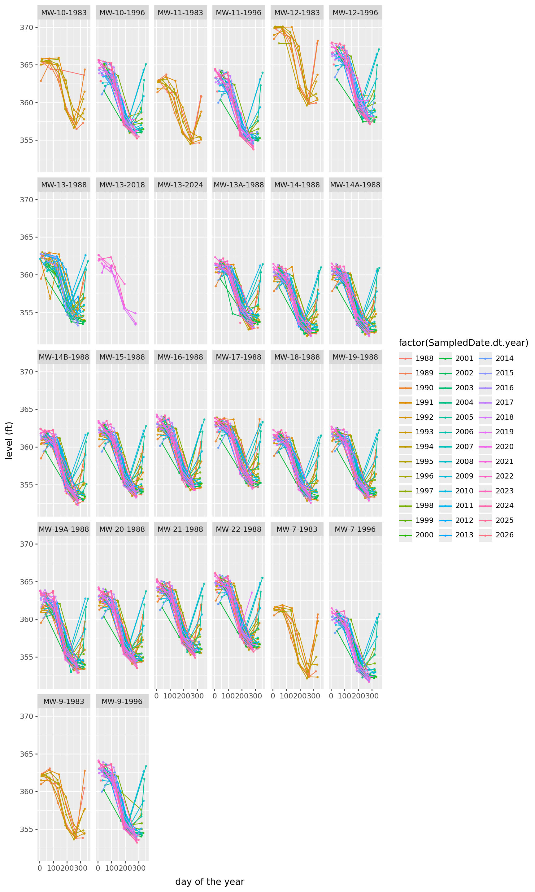
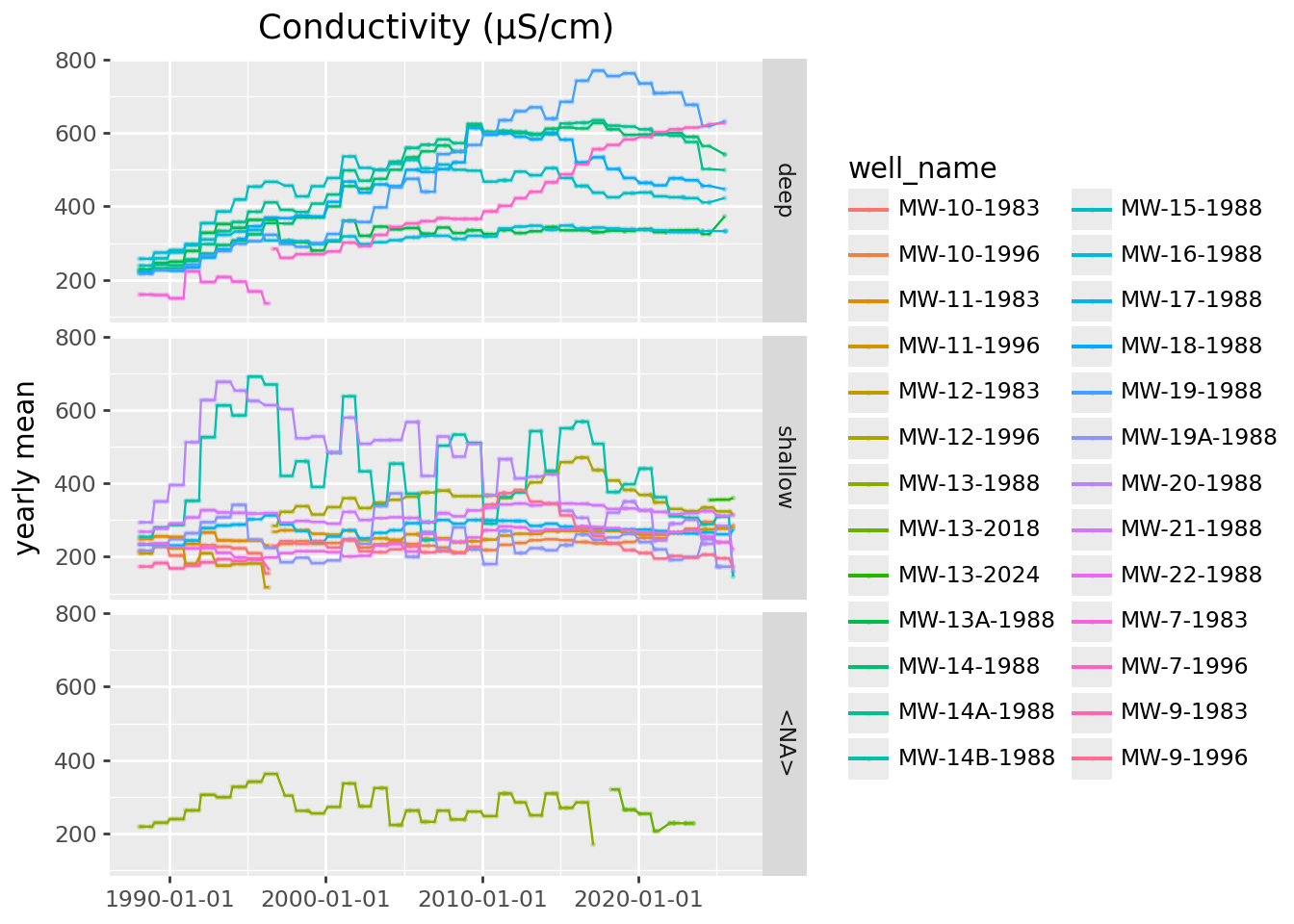
Conductivity
Let’s dive into conductivity:
Does the:
- location relative to the plant,
- or type of well
impact whether it’s:
- increasing/decreasing long term,
- or oscilating.
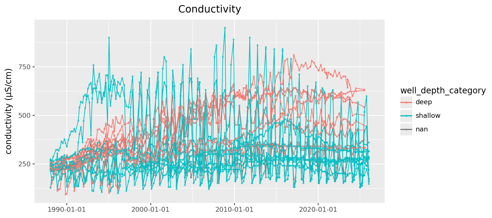
First step: separate out remove seasonal variation.
Model:
value = seasonal + trend(
conductivity
>>
p9.ggplot(p9.aes(x="SampledDate", y="mean_conductivity", color='well_depth_category', group='well_name'))
+ p9.geom_point(size=0.2, alpha=0.25) + p9.geom_line()
+ p9.labs(x='', y='yearly mean', title='Conductivity (µS/cm)')
) / (
conductivity
>>
p9.ggplot(p9.aes(x="SampledDate", y="diff_conductivity", color='well_depth_category', group='well_name'))
+ p9.geom_point(size=0.2, alpha=0.25) + p9.geom_line()
+ p9.labs(x='', y='seasonal difference')
) + p9.theme(figure_size=(9,6))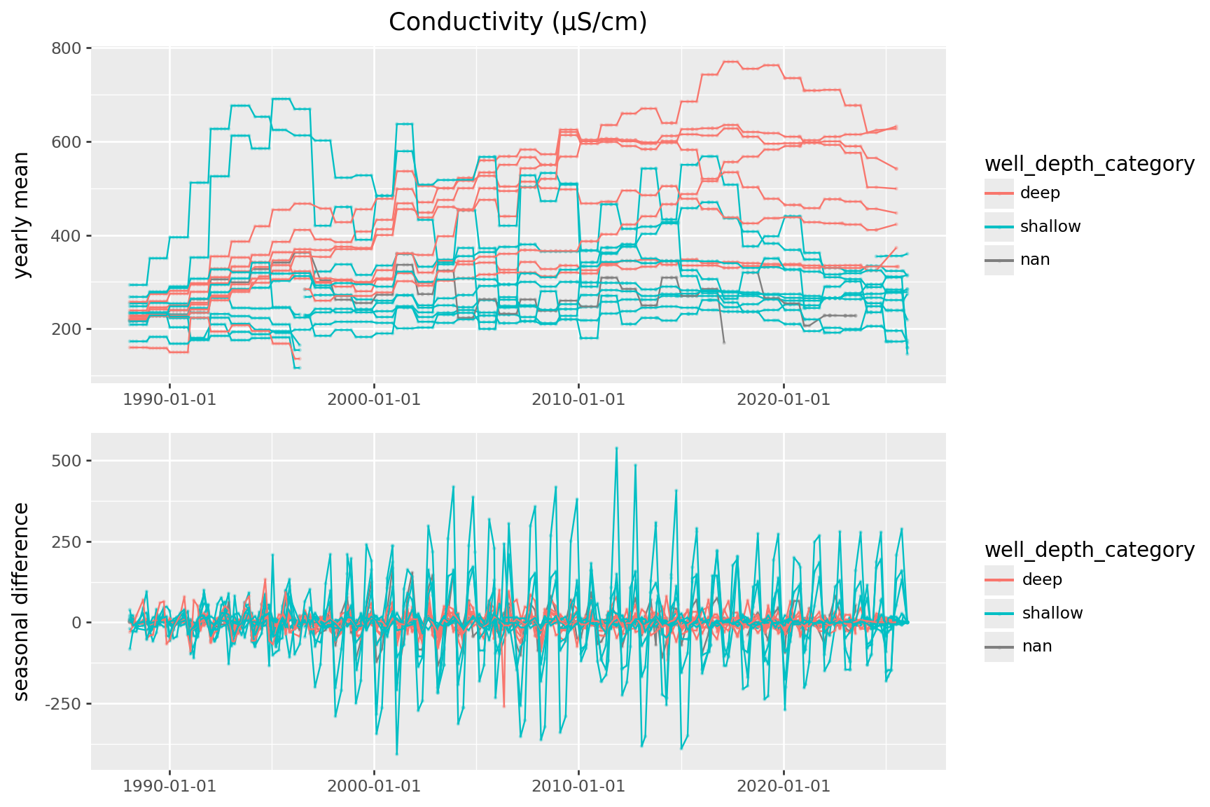
Long-term trends:
Looks like the big increases in conductivity are all at deep wells.