Homework 7: Linear models.

Instructions: Please answer the following questions and submit your work by editing this jupyter notebook and submitting it on Canvas. Questions may involve math, programming, or neither, but you should make sure to explain your work: i.e., you should usually have a cell with at least a few sentences explaining what you are doing.

Also, please be sure to always specify units of any quantities that have units, and label axes of plots (again, with units when appropriate).

import numpy as np
import matplotlib.pyplot as plt
rng = np.random.default_rng(123)

1. Correlation correlation

If $X$ and $Z$ are independent, random Normal with mean 0 and standard deviation 1, and $$\begin{aligned} Y = rX + \sqrt{1 - r^2} Z \end{aligned}$$ then $$ \text{cor}[X, Y] = r . $$

(a) Show that this is true, using math.

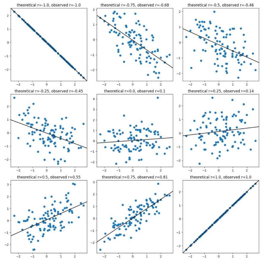
(b) For each of 16 values of $r$ evenly spaced between -1 and 1, simulate 100 draws from a bivariate distribution with correlation $r$. (You should get, for each $r$, 100 pairs $(x_i, y_i)$.) Use these to make a plot like the following (but with four rows and columns), with one scatter plot for each simulation, having the minimum-MSE line superimposed, and both the theoretical and observed correlation in the title.

2. I want candy!

Researchers are planning a study on the effect of children on consumer behavior. In the study, they plan to will record the purchases made by each participants in a month of shopping, and are interested in how the amount spent on candy and other sweets is correlated with the number of children who come along on shopping trips. They have enrolled 65 parents in the study, with the following numbers of accompanying children:

num_children = np.array([0, 0, 0, 0, 0, 0, 0, 0, 0, 0, 0, 0, 0, 0, 0, 1, 1, 1, 1, 1, 1, 1,
       1, 1, 1, 1, 1, 1, 1, 2, 2, 2, 2, 2, 2, 2, 2, 2, 2, 2, 2, 2, 3, 3,
       3, 3, 3, 3, 3, 3, 3, 3, 3, 3, 4, 4, 4, 4, 4, 4, 4, 4, 4, 4, 4])

(Some are zero, for instance, if they have children but none come along when shopping.)

However, they are worried that this small sample size will not allow them to reliably estimate the effect of interest. Your task is to assess this question, by simulation:

(a) Write a function that simulates the amount of sweets purchased from the following model, where $D_i$ is the amount of sweets (in dollars) and $C_i$ is the number of children of the $i^\text{th}$ parent: $$\begin{aligned} X_i &\sim \text{Normal}(\text{mean}= 1 + 5 C_i, \text{sd}=3 C_i) \\ D_i &= \max(0, X_i) . \end{aligned}$$

(b) Simulate one data set, and fit a linear model to these data to predict how the average amount spent on sweets depends on the number of children. You should fit a standard ("least squares") linear model, using either of the methods shown in class: scikit-learn or direct use of the formula. Plot the data with the estimated line on top.

(c) Your result in (b) should have given you estimates of the average amount spent with no children (the intercept), and that the amount increases by, per additional child (the slope). Do the same thing for at least 100 simulated datasets, and make histograms of the resulting estimated slopes and intercepts. How well are these estimated?

3. More mosquitos

Recall the mosquito bite data from HW4: here are the numbers of mosquito bites that 27 kids got on a camping trip:

bites = np.array([4, 5, 4, 2, 4, 8, 4, 6, 7, 5, 4, 0, 5, 7, 5, 3, 2, 0, 3, 4, 5, 3, 6, 1, 2, 3, 5])

Now, we have more data: a parent has measured the concentration of some volatile organics in each kids' breath. Here are the concentrations for the 27 kids (in the same order as bites, above), in units of parts per million (ppm):

odor = np.array([ 2.8,  4.4,  6.9,  2.3,  5.9, 10.2,  3.2,  7.6,  6.3,  4.5,  4.3,
                0. ,  8.2,  5.4,  7.6,  3.3,  3.9,  0.1,  2.7,  4.7,  2.1,  4.3,
               11.3,  1.7,  2.8,  2.9,  8.5])

Our goal is to determine how odor affects the number of bites. To do this, we'll fit a Poisson model: if $Y_i$ is the number of bites the $i^\text{th}$ kid got, and $X_i$ is their "odor" value, then we want to fit: $$\begin{aligned} Y_i \sim \text{Poisson}(\text{mean}= \exp(a X_i + b)) , \end{aligned}$$ i.e., find the values of $a$ and $b$ at which this model best fits the data. To do this:

(a) Write a likelihood function: this should take $a$ and $b$ as arguments, and return the negative log likelihood of the data (i.e., of odor and bites) under the model above.

(b) Use your function from (a) and scipy.optimize.minimize to find the maximum likelihood estimates of $a$ and $b$.

(c) Plot the data, with number of bites against odor, and add the line showing how expected number of bites increases with odor.