Dimension reduction: t-SNE

Peter Ralph

2026-02-04

t-SNE

http://www.jmlr.org/papers/volume9/vandermaaten08a/vandermaaten08a.pdf

t-SNE is a new-er-than-PCA method for dimension reduction (visualization of struture in high-dimensional data).

You can think about this as a lengthy exercise in “let’s dissect a sophisticated loss function for dimension reduction”.

It makes very nice visualizations.

The generic idea is to find a low dimensional representation (i.e., a picture) in which proximity of points reflects similarity of the corresponding (high dimensional) observations.

Suppose we have \(n\) data points, \(x_1, \ldots, x_n\) and each one has \(p\) variables: \(x_1 = (x_{11}, \ldots, x_{1p})\).

For each, we want to find a low-dimensional point \(y\): \[\begin{aligned} x_i \mapsto y_i \end{aligned}\] similarity of \(x_i\) and \(x_j\) is (somehow) reflected by proximity of \(y_i\) and \(y_j\)

We need to define:

“low dimension” (usually, \(k=2\) or \(3\))
“similarity” of \(x_i\) and \(x_j\)
“reflected by proximity” of \(y_i\) and \(y_j\)

Similarity

To measure similarity, we just use (Euclidean) distance: \[\begin{aligned} d(x_i, x_j) = \sqrt{\sum_{\ell=1}^n (x_{i\ell} - x_{j\ell})^2} , \end{aligned}\] after first normalizing variables to vary on comparable scales.

Proximity

A natural choice is to require distances in the new space (\(d(y_i, y_j)\)) to be as close as possible to distances in the original space (\(d(x_i, x_j)\)).

That’s a pairwise condition. t-SNE instead tries to measure how faithfully relative distances are represented in each point’s neighborhood.

Neighborhoods

For each data point \(x_i\), define \[\begin{aligned} p_{ij} = \frac{ e^{-d(x_i, x_j)^2 / (2\sigma^2)} }{ \sum_{\ell \neq i} e^{-d(x_i, x_\ell)^2 / (2 \sigma^2)} } , \end{aligned}\] and \(p_{ii} = 0\).

This is the probability that point \(i\) would pick point \(j\) as a neighbor if these are chosen according to the Gaussian density centered at \(x_i\).

Exercise:

Draw 9 points in a 10m x 10m square. Label the points 1 to 9.
Draw another square, and try to draw the points 1 to 9 in that one so that the neighborhood of point 1 is similar to the first picture, but the neighborhood of point 9 is not.

Reminder: the “neighborhood” is defined by relative distances: for point \(i\) it is \[\begin{aligned} p_{ij} = \frac{ e^{-d(x_i, x_j)^2 / (2\sigma^2)} }{ \sum_{\ell \neq i} e^{-d(x_i, x_\ell)^2 / (2 \sigma^2)} } , \end{aligned}\] and \(p_{ii} = 0\).

Similarly, in the output space, define \[\begin{aligned} q_{ij} = \frac{ (1 + d(y_i, y_j)^2)^{-1} }{ \sum_{\ell \neq i} (1 + d(y_i, y_\ell)^2)^{-1} } \end{aligned}\] and \(q_{ii} = 0\).

This is the probability that point \(i\) would pick point \(j\) as a neighbor if these are chosen according to the Cauchy centered at \(x_i\).

Similiarity of neighborhoods

We want neighborhoods to look similar, i.e., choose \(y\) so that \(q\) looks like \(p\).

To do this, we minimize \[\begin{aligned} \text{KL}(p \;|\; q) &= \sum_{i} \sum_{j} p_{ij} \log\left(\frac{p_{ij}}{q_{ij}}\right) . \end{aligned}\]

What’s KL()?

Kullback-Leibler divergence

\[\begin{aligned} \text{KL}(p \;|\; q) &= \sum_{i} \sum_{j} p_{ij} \log\left(\frac{p_{ij}}{q_{ij}}\right) . \end{aligned}\]

This is the average log-likelihood ratio between \(p\) and \(q\) for a single observation drawn from \(p\).

It is a measure of how “surprised” you would be by a sequence of samples from \(p\) that you think should be coming from \(q\).

Facts:

\(\text{KL}(p \;|\; q) \ge 0\)
\(\text{KL}(p \;|\; q) = 0\) only if \(p_i = q_i\) for all \(i\).

Summary (\(t\)-SNE):

Given data \(\{ x_i \in \mathbb{R}^n \}\), find locations \(\{ y_i \in \mathbb{R}^k \}\) to minimize \[\begin{aligned} \sum_{ij} p_{ij} \log(p_{ij} / q_{ij}) , \end{aligned}\] where \(p_{ij} \propto e^{-d_{ij}^2/\sigma^2}\) and \(q_{ij} \propto 1/(1 + d_{ij}^2)\), and rows in \(p\) and \(q\) are normalized to sum to 1.

Simulate data

set-up

import numpy as np
import pandas as pd
import plotnine as p9
import seaborn as sns
import scipy
import scipy.optimize
rng = np.random.default_rng(seed=123)

A high-dimensional donut

Let’s first make some data. This will be some points distributed around a ellipse in \(n\) dimensions.

n = 20
npts = 1000
xy = rng.normal(size=n*npts).reshape((npts, n))
theta = rng.uniform(size=npts) * 2 * np.pi
theta.sort()
ab = rng.normal(size=2*n).reshape((2, n))
ab[:,1] = ab[:,1] - ab[:,0] * np.sum(ab[:,0] * ab[:,1]) / np.sqrt(np.sum(ab[:,1]**2))
ab /= np.sqrt(np.sum(ab**2, axis=1))[:,np.newaxis]
for k in range(npts):
    dxy = 4 * np.array([np.cos(theta[k]), np.sin(theta[k])]).dot(ab)
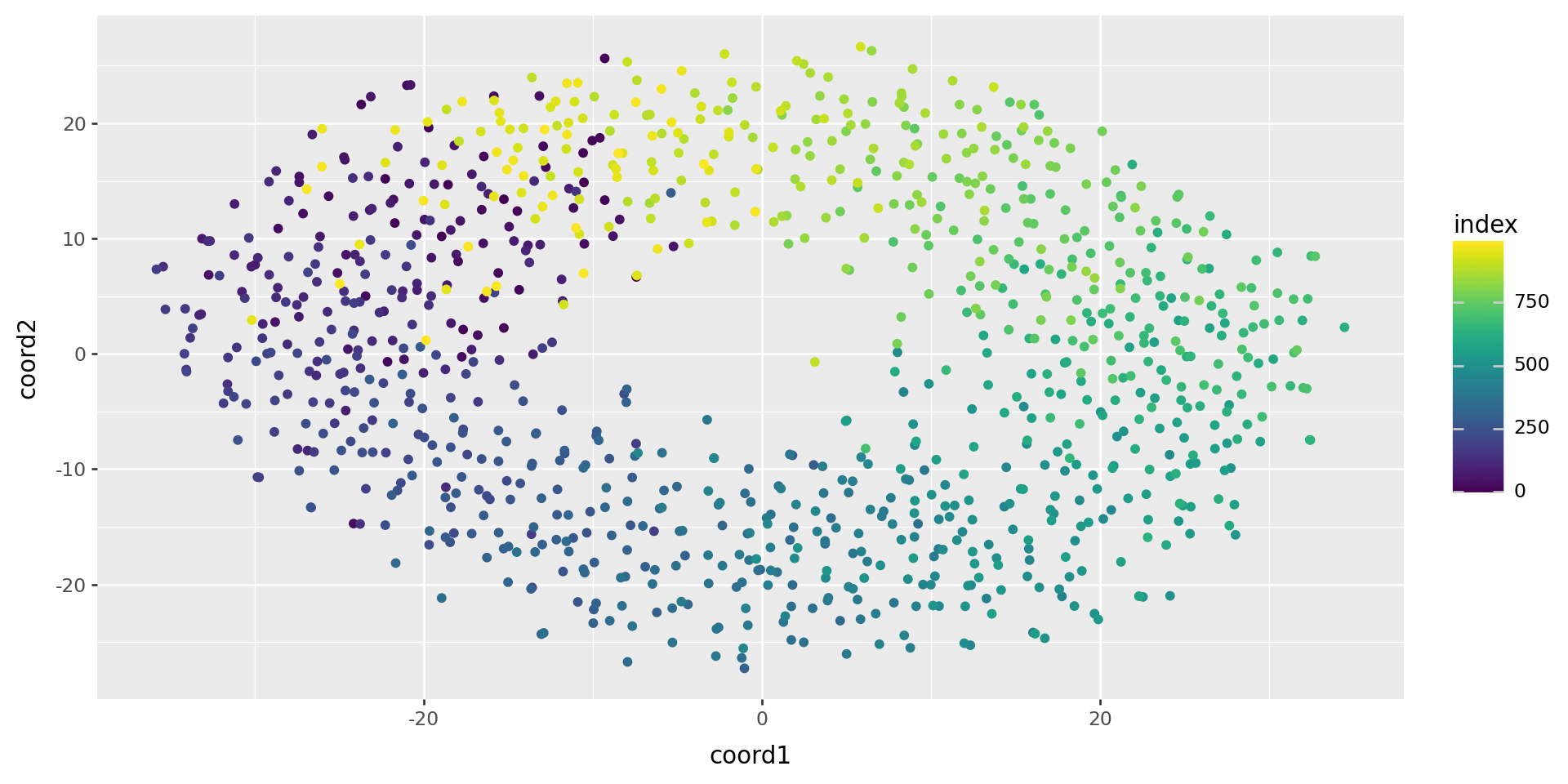
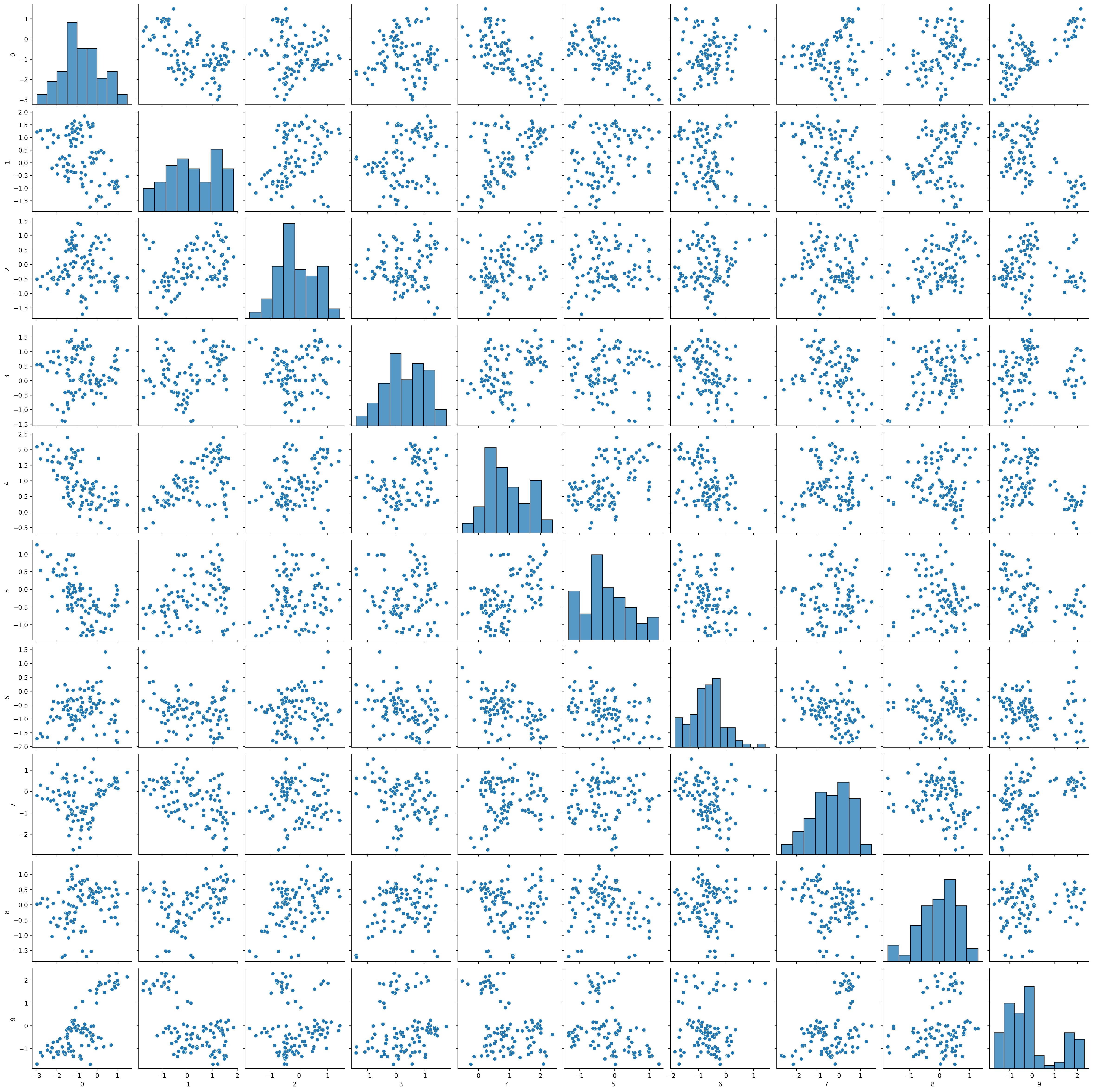
    xy[k,:] += dxy

Here’s what the data look like:

sns.pairplot(pd.DataFrame(xy))

But there is hidden, two-dimensional structure:

(
    pd.DataFrame(xy.dot(ab.T), columns=('a', 'b')).reset_index()
    >>
    p9.ggplot(p9.aes(x='a', y='b', color='index')) + p9.geom_point()
)

Okay, so again:

You could implement \(t\)-SNE, with that description.

But, let’s lean on `skelearn` instead:

import sklearn.manifold
tsne = sklearn.manifold.TSNE(n_components=2).fit_transform(xy)
tsne

array([[-15.271002 ,  13.410212 ],
       [ -7.4323015,   6.672564 ],
       [ -9.591162 ,  18.73543  ],
       ...,
       [-19.885218 ,   1.1804374],
       [ -3.4351227,  16.46511  ],
       [-12.860488 ,  19.459242 ]], shape=(1000, 2), dtype=float32)

It works!

(
    pd.DataFrame(tsne, columns=["coord1", "coord2"]).reset_index()
    >>
    p9.ggplot(p9.aes(x="coord1", y="coord2", color='index'))
    + p9.geom_point()
)

Another case

High-dimensional random walk

n = 40
npts = 100
rw = rng.normal(size=n*npts).reshape((npts, n))
for i in range(1, npts):
    rw[i,:] = np.sqrt(.9) * rw[i-1,:] + np.sqrt(.1) * rw[i,:]

sns.pairplot(pd.DataFrame(rw[:,:10]))

Run again

rw_tsne = sklearn.manifold.TSNE(n_components=2).fit_transform(rw)
rw_tsne

array([[ 5.342569  ,  3.3803456 ],
       [ 5.3078027 ,  3.395333  ],
       [ 5.274957  ,  3.0481176 ],
       [ 5.0061064 ,  2.876894  ],
       [ 4.8534102 ,  2.5876067 ],
       [ 5.2187524 ,  2.218719  ],
       [ 5.326692  ,  2.0201669 ],
       [ 5.35684   ,  1.7662094 ],
       [ 5.116625  ,  1.5398095 ],
       [ 4.971765  ,  1.3300792 ],
       [ 4.5605392 ,  1.5498403 ],
       [ 4.293864  ,  1.3859835 ],
       [ 3.9943395 ,  1.317881  ],
       [ 3.900134  ,  1.7681946 ],
       [ 3.8101308 ,  2.1038268 ],
       [ 3.4808762 ,  2.1810582 ],
       [ 3.048764  ,  1.7975801 ],
       [ 2.7894828 ,  1.9848588 ],
       [ 2.624019  ,  2.0911021 ],
       [ 2.2946653 ,  2.153475  ],
       [ 2.1637692 ,  1.8207891 ],
       [ 2.3605924 ,  1.3225247 ],
       [ 2.249378  ,  1.1781802 ],
       [ 1.5655448 ,  1.2215273 ],
       [ 1.0072862 ,  1.2731194 ],
       [ 0.34624624,  1.2084948 ],
       [ 0.23634873,  1.3298091 ],
       [ 0.06915712,  1.549084  ],
       [-0.21990347,  1.3892608 ],
       [-0.49869773,  1.334521  ],
       [-0.7933359 ,  1.1242819 ],
       [-0.8989207 ,  0.9460818 ],
       [-1.2302965 ,  1.163133  ],
       [-1.6059532 ,  1.4102476 ],
       [-1.9735758 ,  1.3939599 ],
       [-2.2703006 ,  1.1863585 ],
       [-2.6321774 ,  1.1061187 ],
       [-2.8548625 ,  1.7682289 ],
       [-3.0470102 ,  1.8471712 ],
       [-3.279944  ,  1.7185476 ],
       [-3.4666314 ,  1.4054004 ],
       [-3.698554  ,  1.519514  ],
       [-4.040825  ,  1.1959698 ],
       [-4.3375406 ,  0.8117907 ],
       [-4.1977534 ,  0.49342927],
       [-4.2314615 ,  0.2603935 ],
       [-3.9689565 ,  0.11954585],
       [-4.5524664 ,  0.07790056],
       [-4.920539  , -0.01430212],
       [-5.3997974 , -0.39193767],
       [-5.641815  , -0.53180575],
       [-6.0464735 , -1.0483378 ],
       [-6.471822  , -0.93867815],
       [-6.7545137 , -1.0654662 ],
       [-6.9495997 , -1.157594  ],
       [-6.586259  , -1.4898618 ],
       [-6.5522013 , -1.8145885 ],
       [-6.785826  , -2.0510683 ],
       [-7.1808596 , -2.0374916 ],
       [-7.4647293 , -2.2829072 ],
       [-7.639564  , -2.0881324 ],
       [-8.016611  , -2.2220306 ],
       [-8.126271  , -2.646798  ],
       [-8.176487  , -3.18546   ],
       [-8.0286045 , -3.357377  ],
       [-8.052256  , -3.6196513 ],
       [-8.350244  , -4.124479  ],
       [-8.674382  , -4.384362  ],
       [-8.469013  , -4.5470223 ],
       [-8.632379  , -4.7874694 ],
       [-8.6844425 , -5.241904  ],
       [-8.255149  , -5.50136   ],
       [-8.094065  , -5.9435153 ],
       [-7.781794  , -5.6013656 ],
       [-7.475379  , -5.6623573 ],
       [-7.4183664 , -5.824605  ],
       [-7.428164  , -6.278005  ],
       [-7.423861  , -6.6122    ],
       [-7.235864  , -6.948705  ],
       [-7.047818  , -7.278152  ],
       [-7.019246  , -7.4556355 ],
       [-6.817366  , -7.5708995 ],
       [-6.544499  , -7.769315  ],
       [-6.2812705 , -8.029693  ],
       [-5.8719425 , -8.296413  ],
       [-5.5569296 , -8.5241375 ],
       [-5.2331185 , -8.621659  ],
       [-4.8320847 , -8.576095  ],
       [-4.562635  , -8.483491  ],
       [-4.4285564 , -8.403036  ],
       [-4.124957  , -8.507021  ],
       [-3.722636  , -8.76384   ],
       [-3.5903168 , -8.924602  ],
       [-3.2904298 , -8.680731  ],
       [-3.0074747 , -8.432109  ],
       [-2.8198736 , -8.296976  ],
       [-2.5770667 , -8.420178  ],
       [-2.4419682 , -8.5795965 ],
       [-2.4269888 , -8.764668  ],
       [-2.5684159 , -8.945712  ]], dtype=float32)

It works!

(
    pd.DataFrame(rw_tsne, columns=["coord1", "coord2"]).reset_index()
    >>
    p9.ggplot(p9.aes(x="coord1", y="coord2", color='index'))
    + p9.geom_point()
)

Dimension reduction: t-SNE

t-SNE

t-SNE

Similarity

Proximity

Neighborhoods

Similiarity of neighborhoods

Kullback-Leibler divergence

Summary (\(t\)-SNE):

Simulate data

set-up

A high-dimensional donut

Okay, so again:

But, let’s lean on skelearn instead:

It works!

Another case

High-dimensional random walk

Run again

It works!

But, let’s lean on `skelearn` instead: