Spatial smoothing

Peter Ralph

2026-02-25

Spatial point data: Biketown

Albert in a bike (catmapper:Wikimedia)

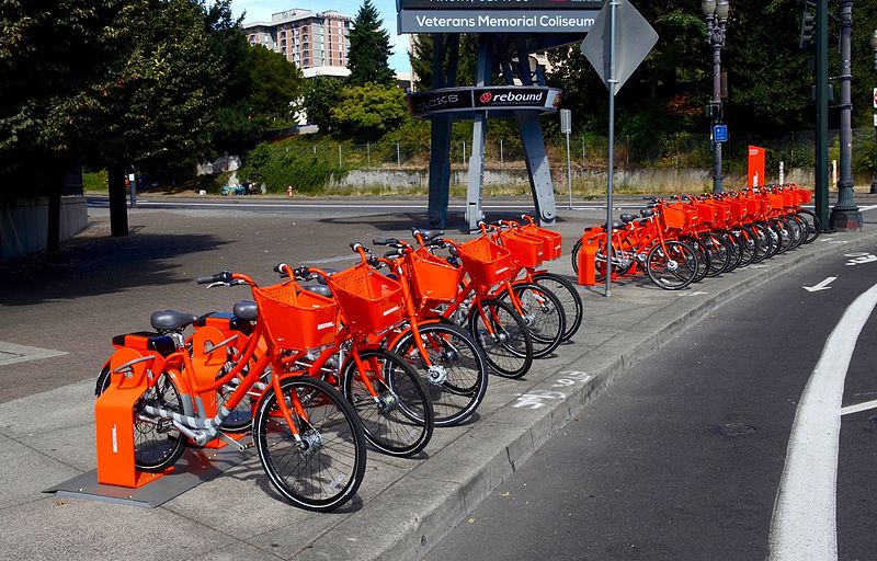
biketown bikes (Steve Morgan: Wikimedia)

how biketown works: screenshot

import pyproj
import geopandas as gpd
import pandas as pd
import numpy as np
import scipy.ndimage
import matplotlib.pyplot as plt
import contextily

August, 2018

Here is data from August, 2018.

df = pd.read_csv("data/biketown/2018_08.csv.gz")
df = df.loc[~df['StartLatitude'].isna(),:]
df.head(n=5)

	RouteID	PaymentPlan	StartHub	StartLatitude	StartLongitude	StartDate	StartTime	EndHub	EndLatitude	EndLongitude	EndDate	EndTime	TripType	BikeID	BikeName	Distance_Miles	Duration	RentalAccessPath	MultipleRental
0	8530077	Casual	NW Couch at 11th	45.523742	-122.681813	8/1/2018	0:00	NE Couch at MLK	45.523588	-122.661918	8/1/2018	0:09	NaN	6841	0075 BIKETOWN	1.09	0:08:41	mobile	False
1	8530088	Casual	NE Couch at MLK	45.523588	-122.661918	8/1/2018	0:01	SW 2nd at Pine	45.521421	-122.672629	8/1/2018	0:08	NaN	7312	0987 BETRUE TRAINER	0.62	0:07:24	mobile	False
2	8530156	Subscriber	SW 3rd at Ankeny	45.522479	-122.673297	8/1/2018	0:07	NaN	45.522987	-122.681129	8/1/2018	0:31	NaN	6145	0567 BIKETOWN	2.62	0:23:36	keypad	False
3	8530170	Subscriber	NaN	45.520015	-122.682115	8/1/2018	0:08	NaN	45.536330	-122.685748	8/1/2018	0:18	NaN	7498	0181 BIKETOWN	1.36	0:09:51	keypad_rfid_card	False
4	8530168	Subscriber	NaN	45.520015	-122.682115	8/1/2018	0:08	NaN	45.536330	-122.685748	8/1/2018	0:18	NaN	6879	0747 BIKETOWN	1.36	0:09:39	keypad_rfid_card	False

Transform points

First, we’d like actual spatial points in a sensible (isometric) coordinate system:

df['start_points'] = gpd.points_from_xy(df.StartLongitude, df.StartLatitude, crs="EPSG:4326").to_crs("EPSG:5070")
df['end_points'] = gpd.points_from_xy(df.EndLongitude, df.EndLatitude, crs="EPSG:4326").to_crs("EPSG:5070")
gdf = gpd.GeoDataFrame(df, geometry=df['start_points'], crs=5070)
gdf[:1000].explore()

Make this Notebook Trusted to load map: File -> Trust Notebook

Goals

1. Where do most trips start?
2. Where do they end up?
3. Is there a net flux of bikes anywhere?

We’ll make some maps with spatial smoothing to answer this, and evaluate if that was a good tool for the job.

Interlude: when there’s lots of data

Too much data?

In this class we’ve mostly not worried about computation. Modern computers deal with vectors of length \(10^7\)–\(10^8\) pretty much instantly.

But, what if you’ve got more? Options:

1. Use less data.
2. Look at summaries of the data.

Considerations:

• Do you really need \(n=10^{12}\) for whatever you’re looking for? Probably not!
• If you sub-sample, make sure the sub-sampling is appropriate (i.e., if the sub-sample has structure, it’s structure you want to look at).
• You probably want to pilot your summaries on a sub-sample anyhow.

Too much data, take two

It’s real easy to run into “too much data” in spatial contexts, basically because \(N^2 > N\).

Why?

• Images/rasters: my display is 2256 x 1504, which is 3.3M pixels. It’s easy to have a lot of images.

• Pairwise comparisons: Many spatial operations require operating “nearby” objects. Naively, that requires working with all \(O(N^2)\) pairwise distances.

Example: kernel density estimation

Suppose we have a bunch of points

\[ (x_1, y_1), \ldots, (x_n, y_n) \]

with density \(f(x,y)\), i.e.,

\[ f(x,y) \approx \frac{\#(\text{of points within $r$ of $(x,y)$})}{\pi r^2} \]

Using (for instance)

\[ \rho_\sigma(x,y) = \frac{1}{2\pi\sigma^2} e^{-\frac{x^2+y^2}{2\sigma^2}} \]

we can estimate \(f(x,y)\) by

\[ \hat f(x,y) = \sum_{i=1}^n \rho_\sigma(x_i-x, y_i-y) . \]

(interlude: why?)

Try it out (in one dimension)

1. Simulate 200 spatial locations with a density having two “bumps”. Plot these points. (rng.normal(size=n, loc=-3), rng.normal(size=n, loc=+3))

2. Make 20 “reference” locations.

3. Compute the kernel density estimate for each reference location, with \(\sigma\) chosen appropriately, and plot it. (scipy.stats.norm( ))

Uh-oh, it’s quadratic

Note that this required \(O(NM)\) operations, where \(N\) is the number of data points, and \(M\) is the number of reference locations.

This is not as bad as \(O(N^2)\)!

But, suppose we wanted “density estimate for each of our \(N\) points”. The naive method would use data points = reference points: \(O(N^2)\).

Better: get estimated density at a grid of references, and use linear interpolation.

Guidelines for keeping your computer happy

• Start with small \(N\), look out for things that take a long time.
• If you actually need “all pairwise” values, keep \(N\) small (below 1,000 or so?).
• If an operation seems to need pairwise values under the hood, use “algorithms”: for instance, \(k-d\) trees (spatial libraries will do this sort of thing for you).

Back to the data

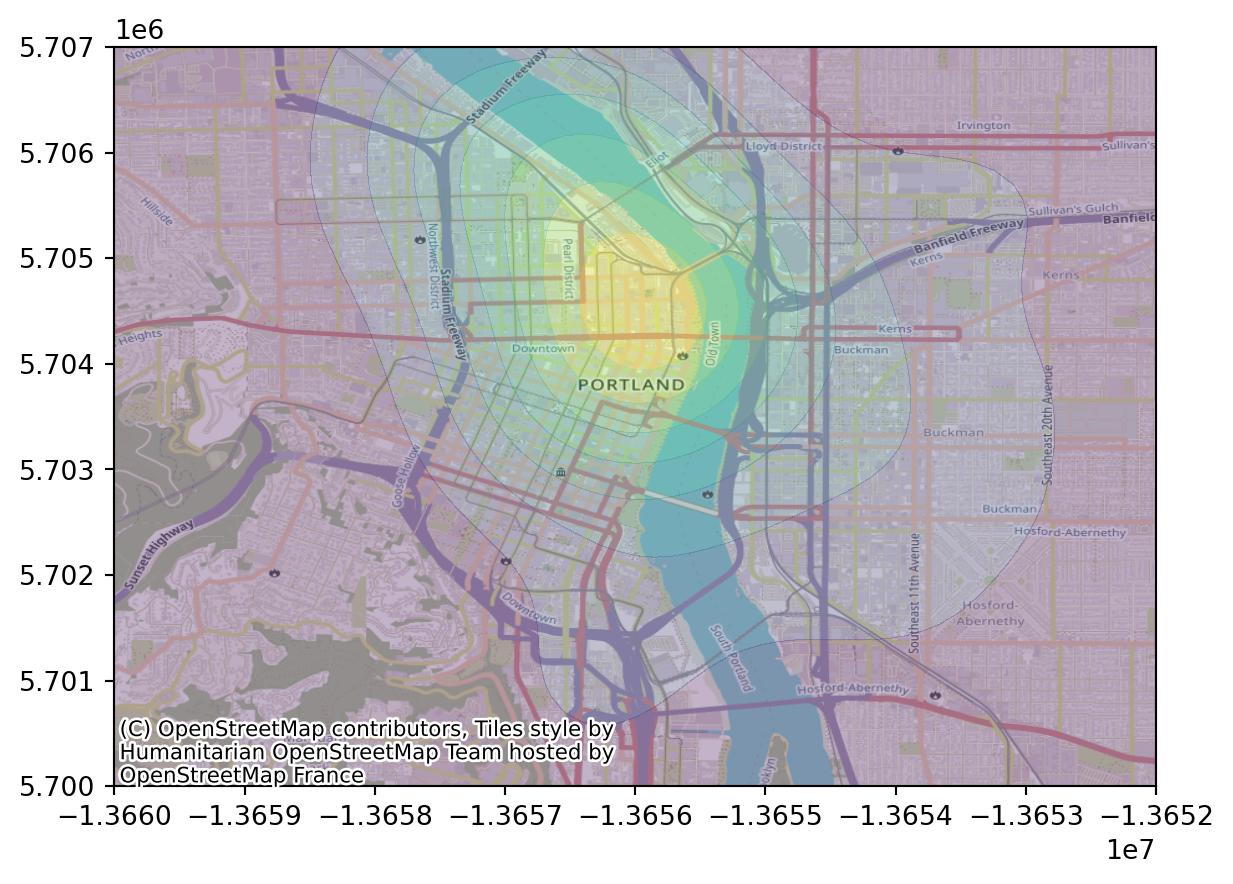
Smoothed map of starting locations

First, we’ll bin things into a 2D grid:

sigma = 500 # meters
delta = 100 # meters
xy = np.array([x.coords[0] for x in gdf['start_points']])
extent = [np.min(xy[:,1]), np.max(xy[:,1]), np.min(xy[:,0]), np.max(xy[:,0])]
xx = np.linspace(extent[2], extent[3], int(abs(extent[3]-extent[2])/delta))
yy = np.linspace(extent[0], extent[1], int(abs(extent[1]-extent[0])/delta))
heatmap, xedges, yedges = np.histogram2d(xy[:,0], xy[:,1], bins=[xx, yy])
plt.imshow(heatmap)

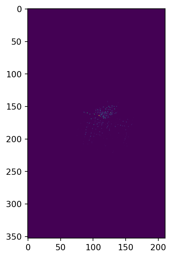
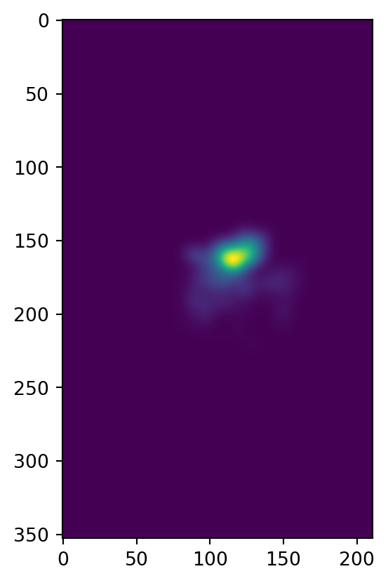
Then, we smooth it: (question: how’s this relate to how we did KDE above?)

heatmap = scipy.ndimage.gaussian_filter(heatmap, sigma=sigma/delta, mode='nearest')
plt.imshow(heatmap)

Better plotting

There’s various ways to do this. One is to use contextily as demonstrated here. First, we need to convert to “EPSG:3857 (Web Mercator)”:

xpts = gpd.points_from_xy(xx, np.full((len(xx),), np.mean(yy)), crs="EPSG:5070").to_crs("EPSG:3857")
ypts = gpd.points_from_xy(np.full((len(yy),), np.mean(xx)), yy, crs="EPSG:5070").to_crs("EPSG:3857")
gpd.GeoDataFrame(geometry=gpd.points_from_xy(
    np.concat([xx, np.full((len(yy),), np.mean(xx))]), 
    np.concat([np.full((len(xx),), np.mean(yy)), yy])),
    crs="EPSG:5070").to_crs("EPSG:3857").explore()

Make this Notebook Trusted to load map: File -> Trust Notebook

Now, we can superimpose on the OSM map:

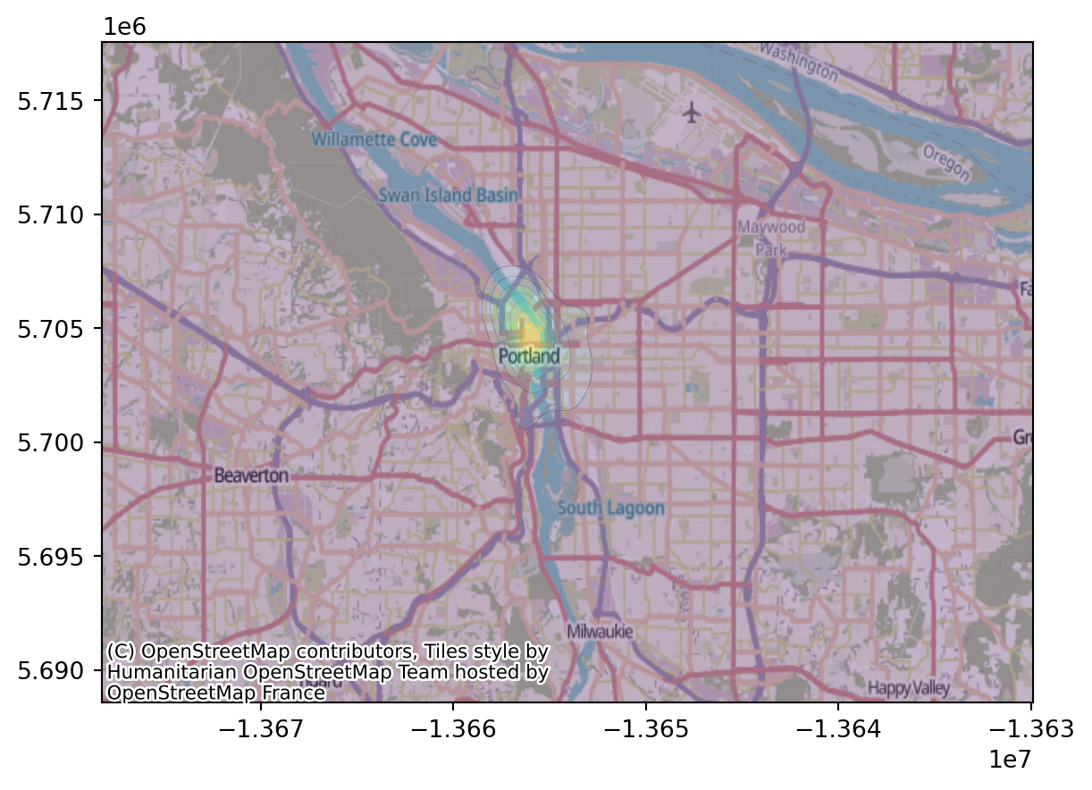
XX, YY = np.meshgrid(
    [x.coords[0][0] for x in xpts[1:]],
    [y.coords[0][1] for y in ypts[1:]],
)
fig, ax = plt.subplots()
ax.contourf(XX, YY, heatmap.T, alpha=0.3)
contextily.add_basemap(ax);

Let’s zoom in:

fig, ax = plt.subplots()
ax.contourf(XX, YY, heatmap.T, alpha=0.3)
ax.set_xlim(-1.366e7, -1.3652e7)
ax.set_ylim(5.7e6, 5.707e6)
contextily.add_basemap(ax);

Bandwidth is important

Question:

Above I set:

sigma = 500 # meters
delta = 100 # meters

What are these numbers, in words, and are these good choices?

Exercise:

Explore different choices of these two parameters. To do this:

1. Write a function that takes in sigma and delta and makes a plot.
2. Play around with it.

Choosing a bandwidth

How to pick a bandwidth?

There are various automatic methods.

But… crossvalidation!

For each bandwidth:

1. Fit using most of the data,
2. and predict the remaining data.
3. Do this a bunch and return an estimate of goodness-of-fit.

… but wait, what’s this mean, here?

Revised:

For each bandwidth:

1. Fit the smooth using most of the data,
2. predict the density at the locations of the remaining data,
3. and return the mean log density at “true” points.

Why log?:

If \(f\) and \(g\) are probability distributions, and \(x_1, \ldots, x_n\) are drawn from \(f\), then \[ L(g) = \sum_{i=1}^n \log g(x_i) \lessapprox L(f) , \] i.e., is maximized for \(g=f\). (see: cross entropy)