Mapping with the census
2026-02-23
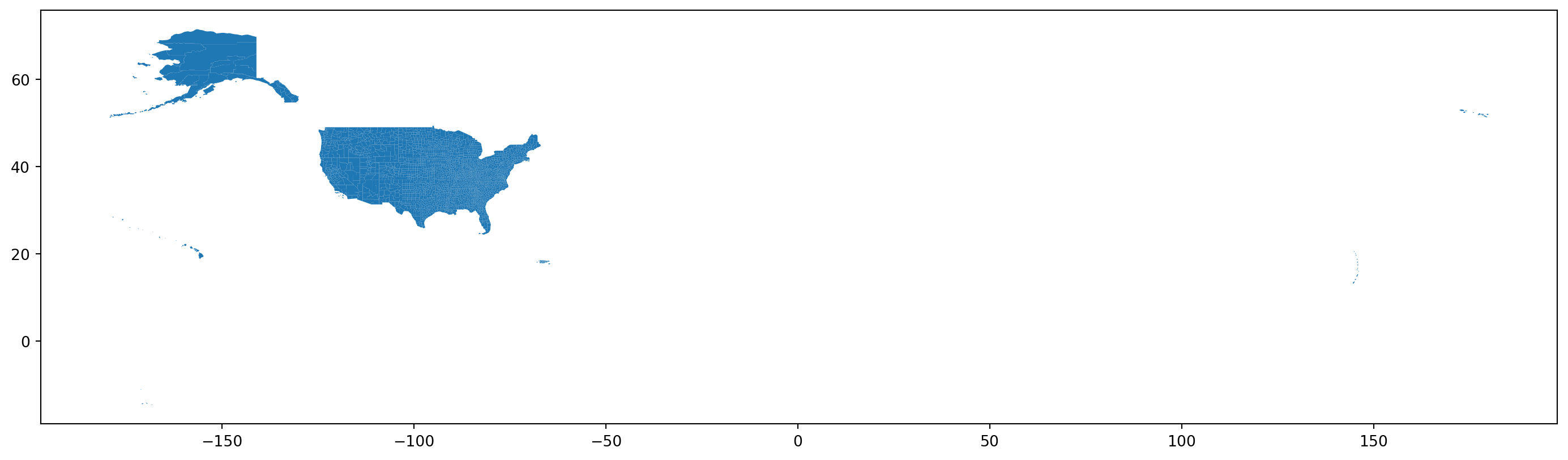
What’s in there?
Geopandas uses shapely:

Here’s the best part, though:
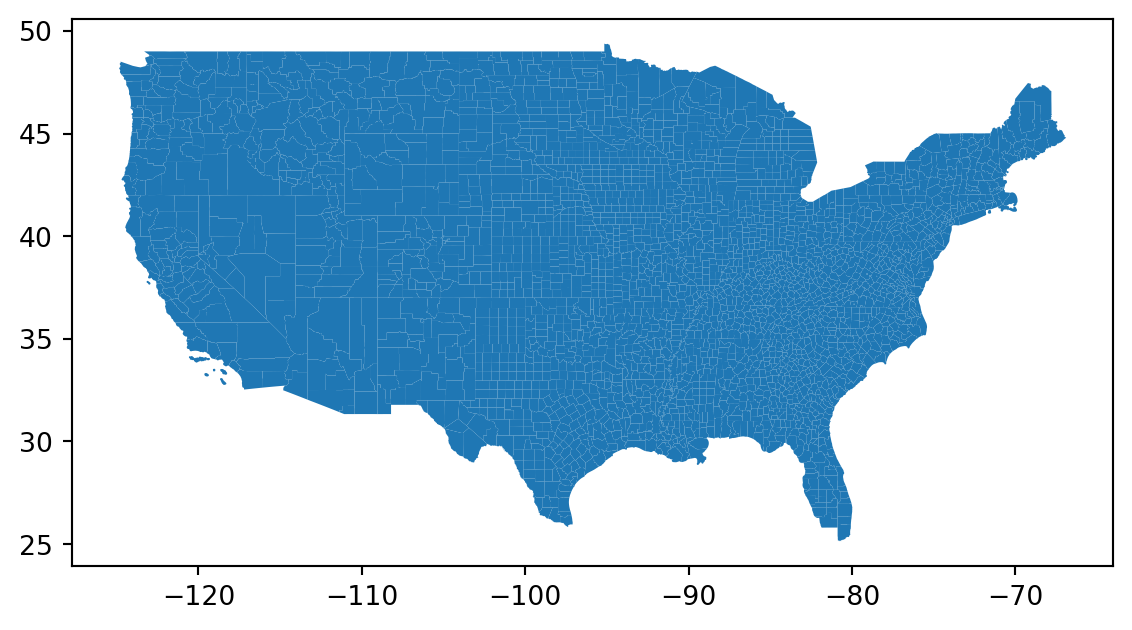
Subset to a bounding box:
.cx: Coordinate based indexer to select by intersection with bounding box.
Finding “bounding box for contiguous USA” gives these coordinates, used in .cx
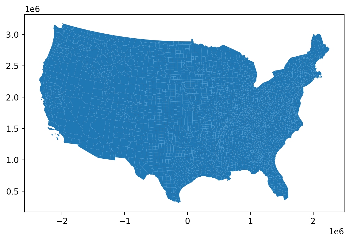
Equal area:
Let’s use the Albers equal area for the contiguous US: EPSG:5070
Where do the people live?
First try: critiques?
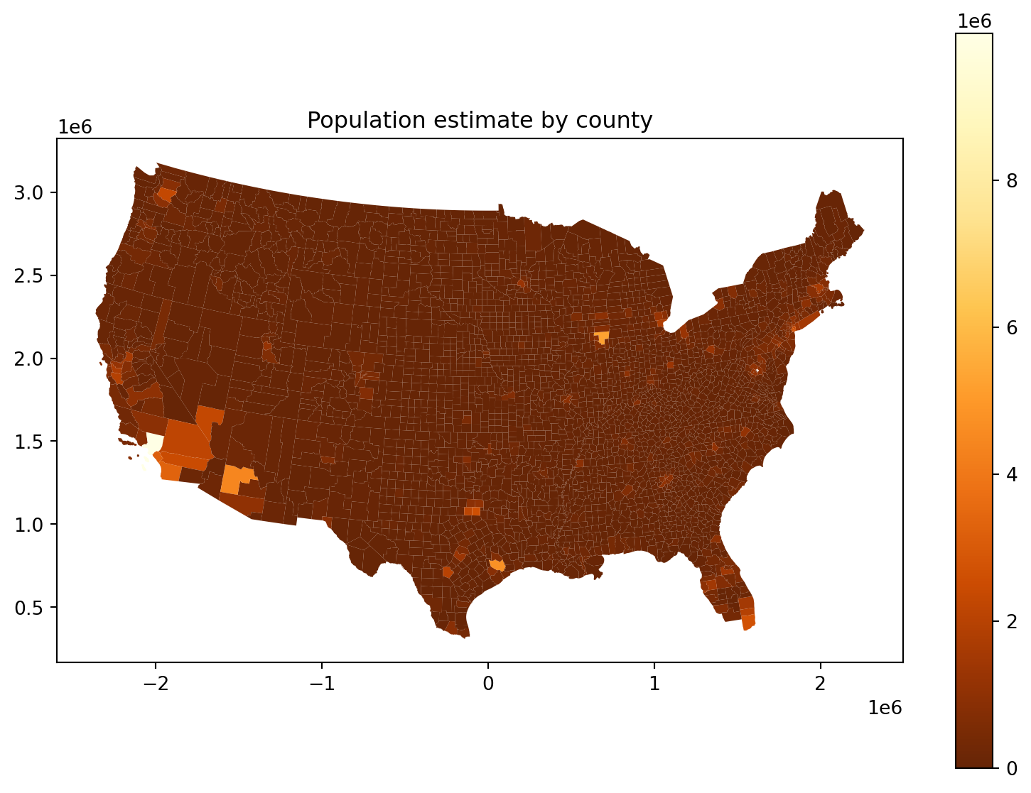
The problem:
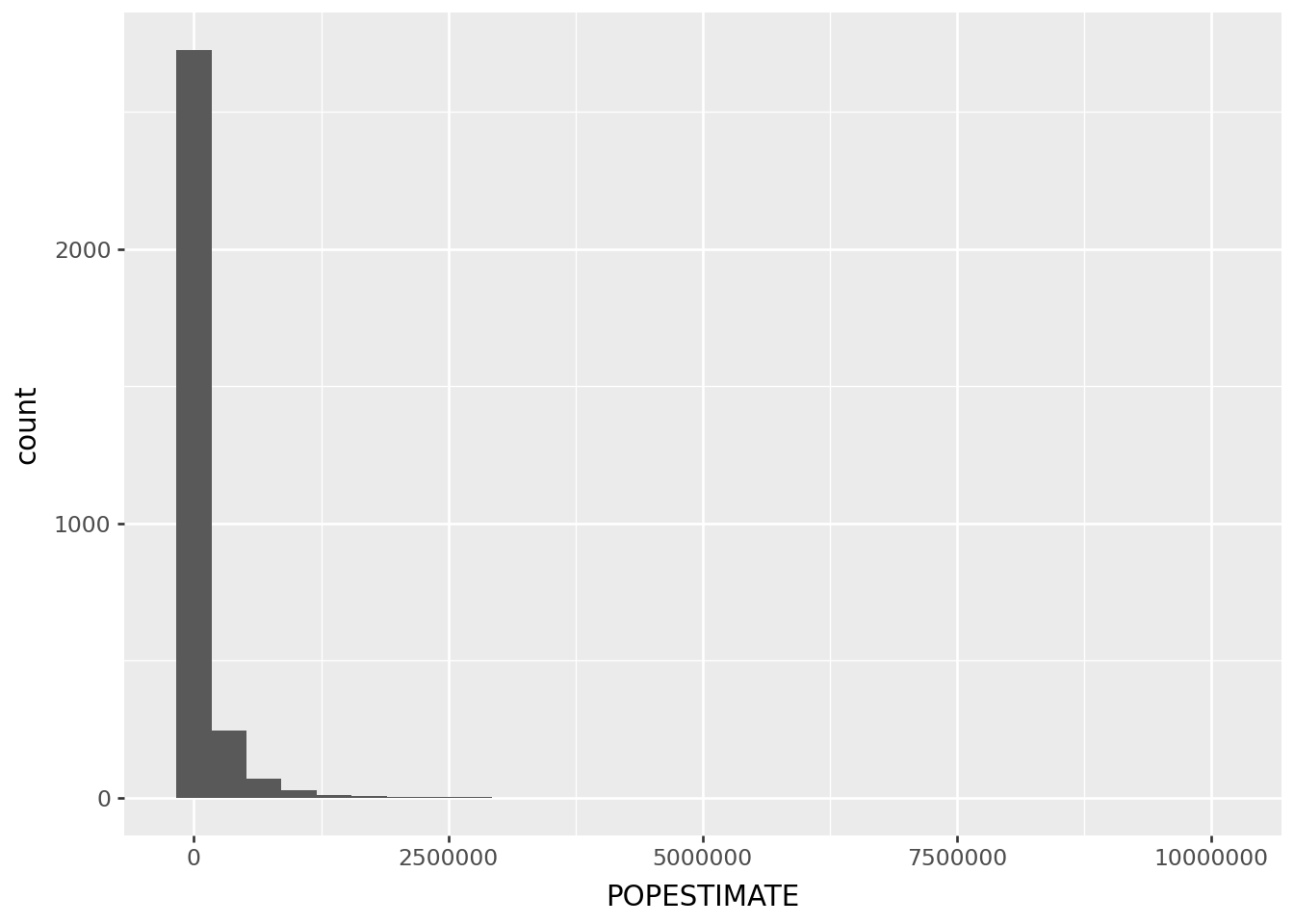
Where do the people live, take 2:
Log scale:
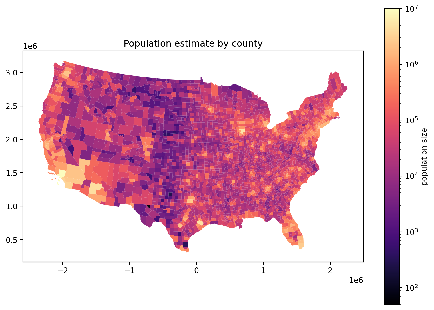
Where do the people live, take 3:
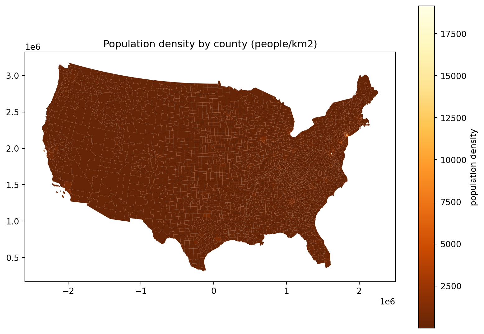
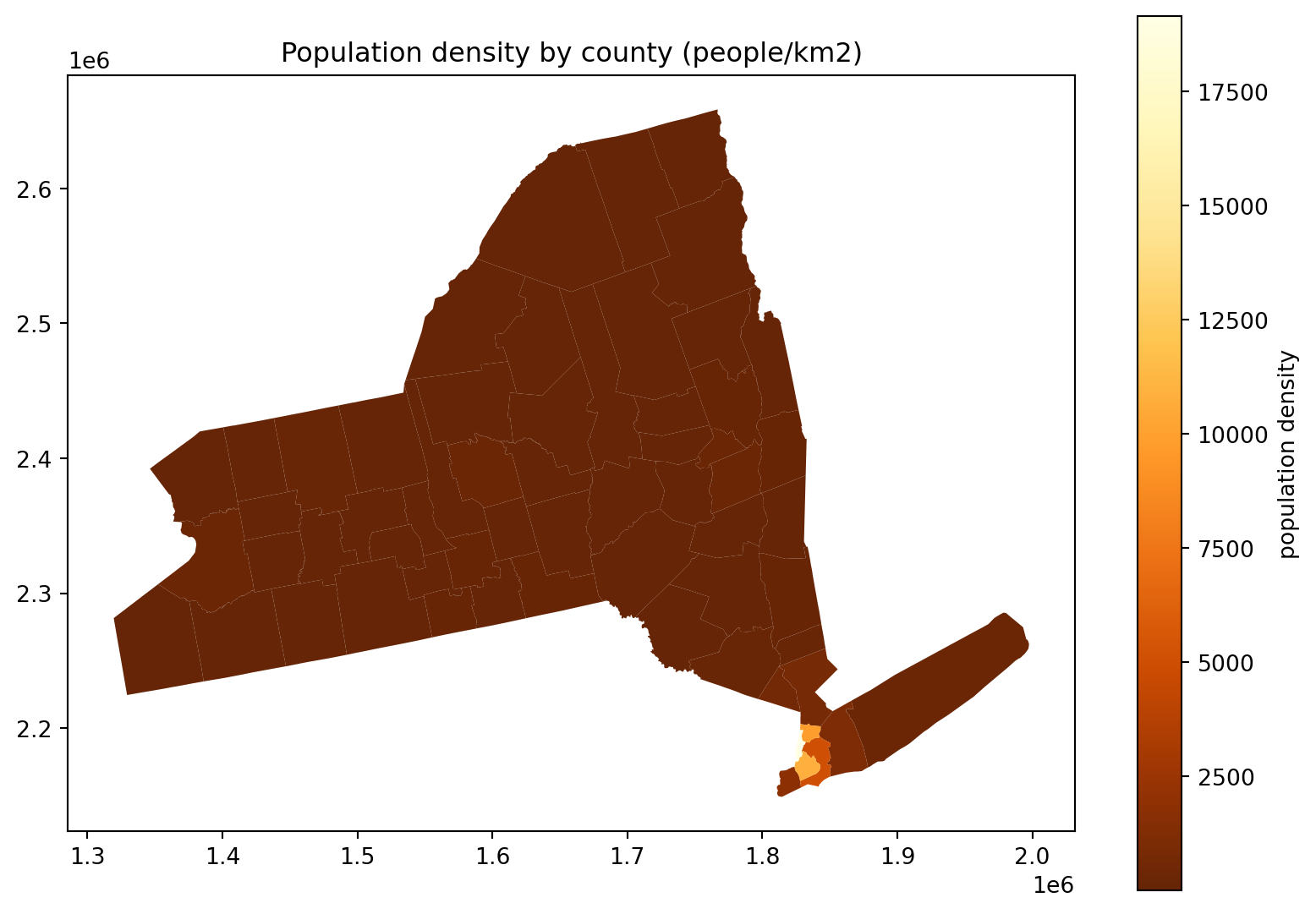
Hm, where’s all the people in this plot?
fig, ax = plt.subplots(1, 1, figsize=(10, 7))
ax.set_title("Population density by county (people/km2)")
(
    cdf
    .query("STNAME == 'New York'")
    .assign(density=lambda df: df['POPESTIMATE']*1e6/df['geometry'].area)
    .plot(column='density', legend=True, ax=ax, legend_kwds={'label': 'population density'}, cmap='YlOrBr_r')
);
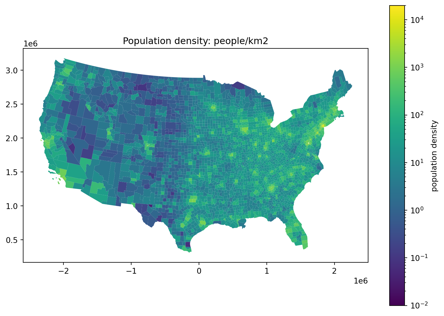
Where do the people live, take 4:
fig, ax = plt.subplots(1, 1, figsize=(10, 7))
ax.set_title("Population density: people/km2")
(
    cdf
        .assign(density=lambda df: df['POPESTIMATE']*1e6/df['geometry'].area)
        .plot(column='density', legend=True, ax=ax,
              norm=matplotlib.colors.LogNorm(vmin=0.01, vmax=2e4),
              legend_kwds={'label': 'population density'},
        )
);
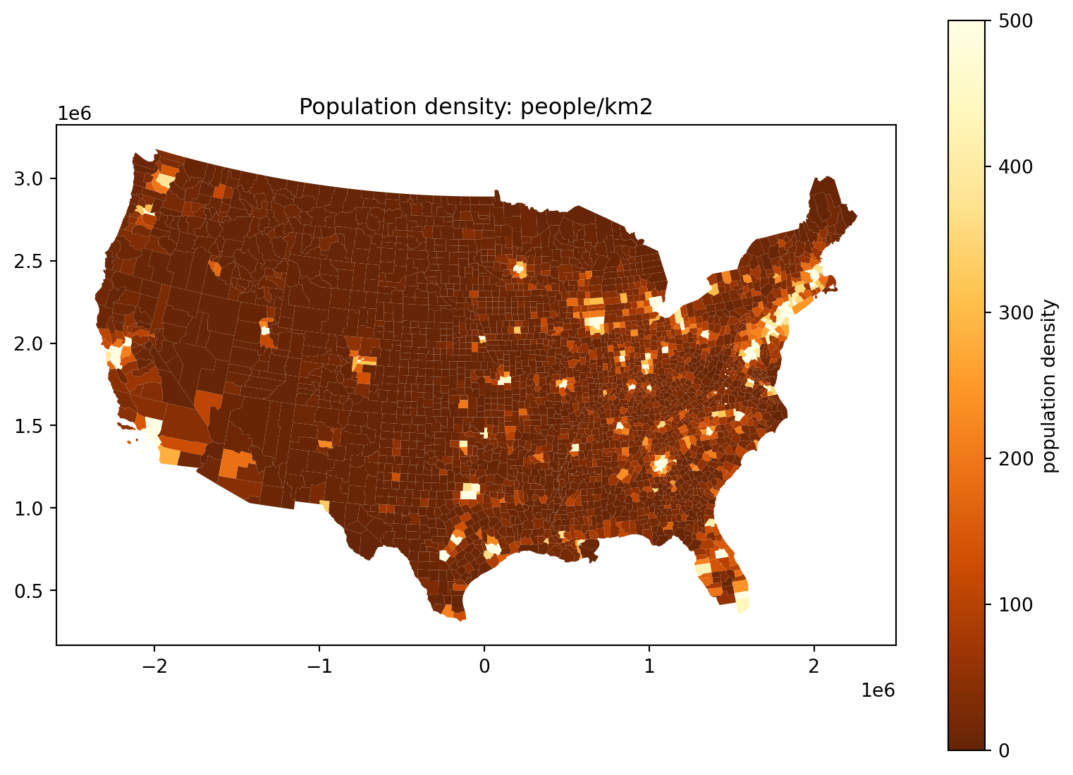
Where do the people live, take 5:
Alternatively, we could truncate:
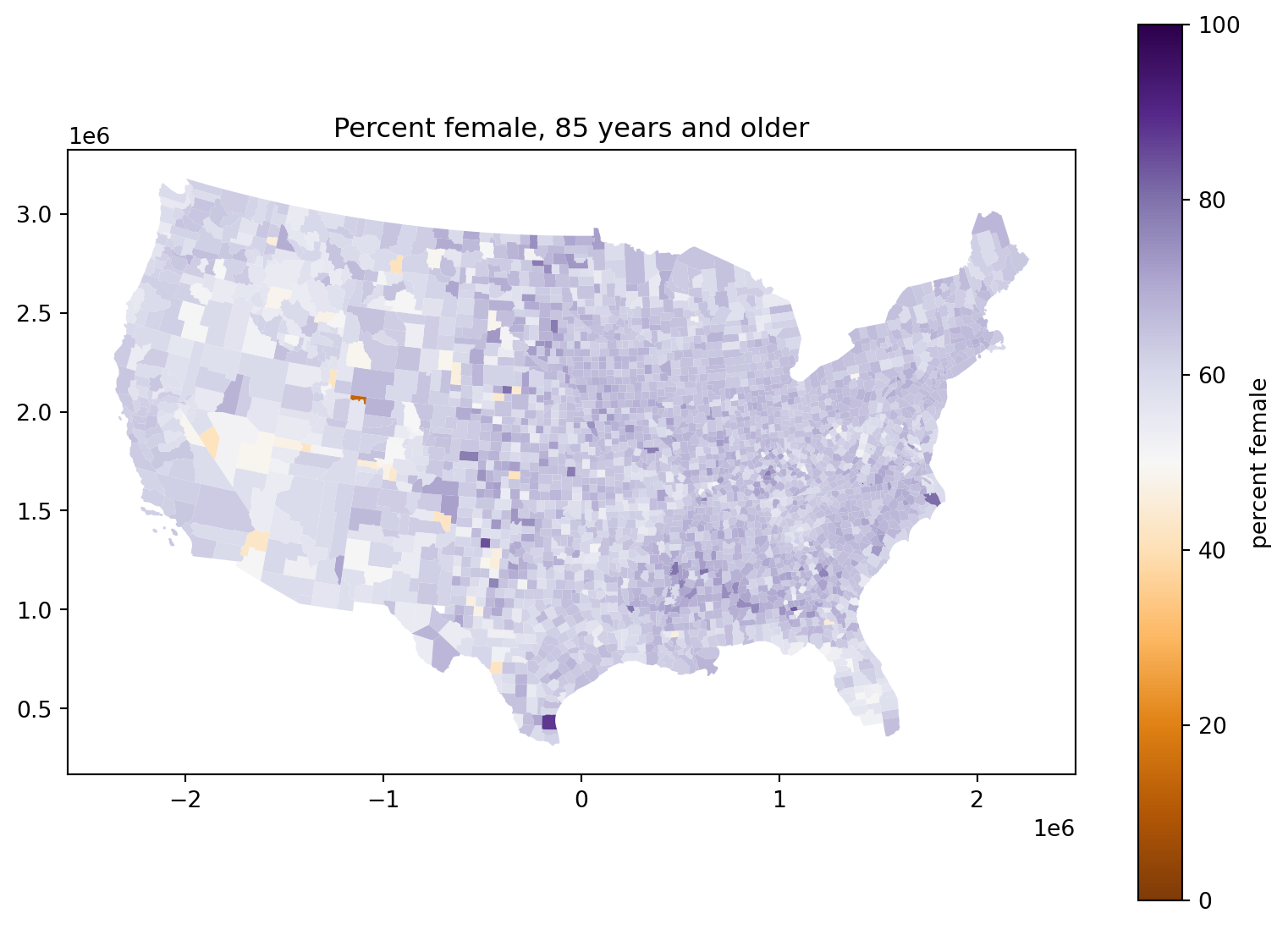
Percent female, 85 years and older:
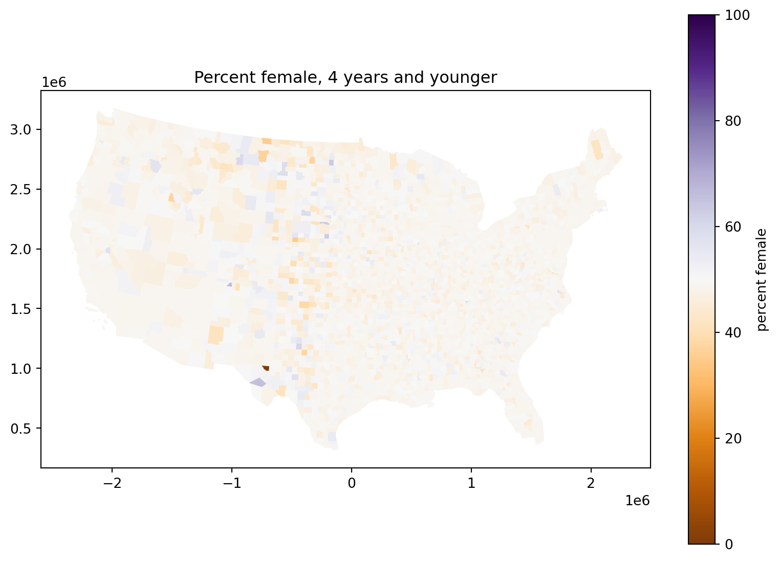
Percent female, 4 years and younger:
What’s going on with those counties in the middle of the country?
Exercise: debunk yourself
Come up with a wild explanation for why counties in the middle of the country tend to have a sex ratio at birth that is farther from 50%.
Explain why it’s not supported by the data.

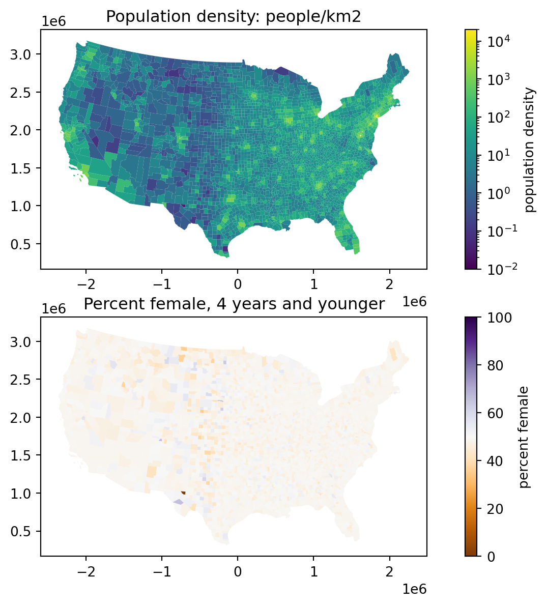
Okay but what is going on?
Consider:
fig, (ax1, ax2) = plt.subplots(2, 1, figsize=(10, 7))
ax1.set_title("Population density: people/km2")
(
    cdf .assign(density=lambda df: df['POPESTIMATE']*1e6/df['geometry'].area)
        .plot(column='density', legend=True, ax=ax1,
              norm=matplotlib.colors.LogNorm(vmin=0.01, vmax=2e4),
              legend_kwds={'label': 'population density'},)
);
ax2.set_title("Percent female, 4 years and younger")
(
    cdf .assign(pfem=100*cdf['AGE04_FEM']/cdf['AGE04_TOT'])
        .plot(column='pfem', legend=True, ax=ax2,
              legend_kwds={'label': 'percent female'},
              cmap='PuOr', vmin=0, vmax=100,)
);
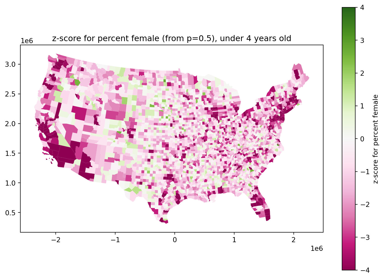
Are newborn sex ratios even?
They look definitely skewed male:
fig, ax = plt.subplots(1, 1, figsize=(10, 7))
ax.set_title(f"z-score for percent female (from p=0.5), under 4 years old")
(
    cdf
        .assign(
            z = lambda df: (df['AGE04_FEM'] - 0.5 * df['AGE04_TOT']) / np.sqrt(0.5 * (1-0.5) * df['AGE04_TOT']),
        )
        .plot(column='z', legend=True, ax=ax,
              legend_kwds={'label': 'z-score for percent female'},
              cmap='PiYG', vmin=-4, vmax=4,
        )
);
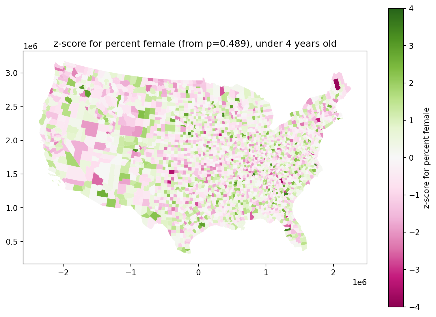
Do newborn sex ratios differ across the country?
They look definitely skewed male:
total_pfem = cdf['AGE04_FEM'].sum() / cdf['AGE04_TOT'].sum()

fig, ax = plt.subplots(1, 1, figsize=(10, 7))
ax.set_title(f"z-score for percent female (from p={total_pfem:.3}), under 4 years old")
(
    cdf
        .assign(
            z = lambda df: (df['AGE04_FEM'] - total_pfem * df['AGE04_TOT']) / np.sqrt(total_pfem * (1-total_pfem) * df['AGE04_TOT']),
        )
        .plot(column='z', legend=True, ax=ax,
              legend_kwds={'label': 'z-score for percent female'},
              cmap='PiYG', vmin=-4, vmax=4,
        )
);
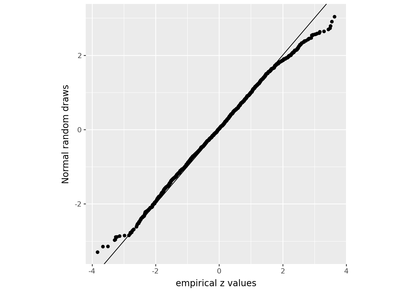
Are they bigger than we’d expect?
Here’s a low-tech QQ plot:
rng = np.random.default_rng(seed=123)

z = (
    cdf.assign(
        z=lambda df: (df['AGE04_FEM'] - total_pfem * df['AGE04_TOT']) / np.sqrt(total_pfem * (1-total_pfem) * df['AGE04_TOT'])
    )
    .sort_values("z")
)[['NAME', 'STNAME', 'z', 'AGE04_FEM', 'AGE04_MALE', 'AGE04_TOT']]

(
    z.assign(znorm = np.sort(rng.normal(size=len(z))))
    >>
    p9.ggplot(p9.aes(x='z', y='znorm'))
    + p9.geom_point()
    + p9.labs(x='empirical z values', y='Normal random draws')
    + p9.theme(aspect_ratio=1.0)
    + p9.geom_abline(slope=1, intercept=0)
)
/home/peter/micromamba/envs/ds435/lib/python3.13/site-packages/plotnine/layer.py:374: PlotnineWarning: geom_point : Removed 1 rows containing missing values.