Landsat images
2026-03-02
The NASA/USGS Landsat program provides the longest continuous space-based record of Earth’s land in existence. Landsat data are essential for making informed decisions about our planet’s resources and environment.

Data (Landsat 8/9):
- 700 scenes/day, 185km wide
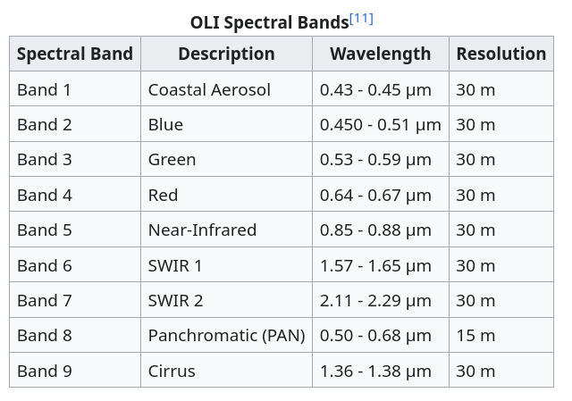
- 11 spectral bands from a multispectral scanner
- 15m/30m/100m pixels

Obtaining the data
It’s free: from earthexplorer.usgs.gov
as GeoTIFF raster files
and there’s a LOT of it: each scene is ~1G
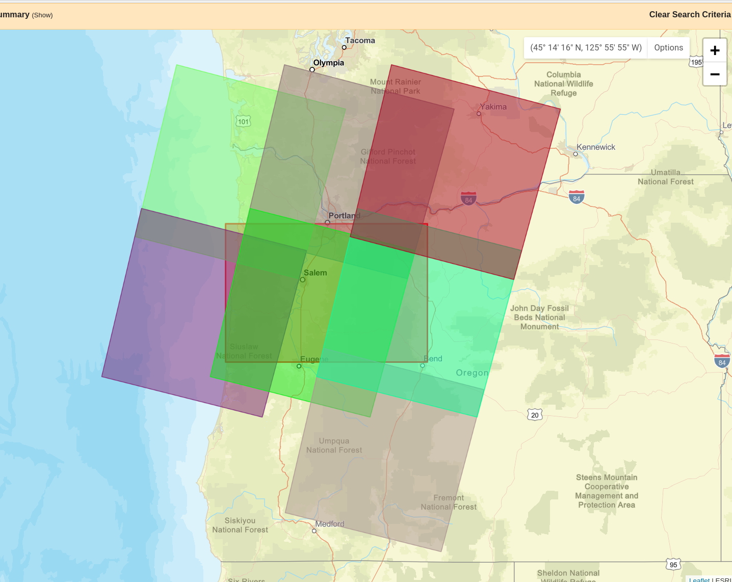
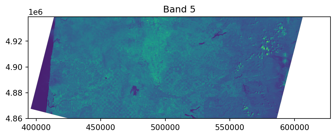
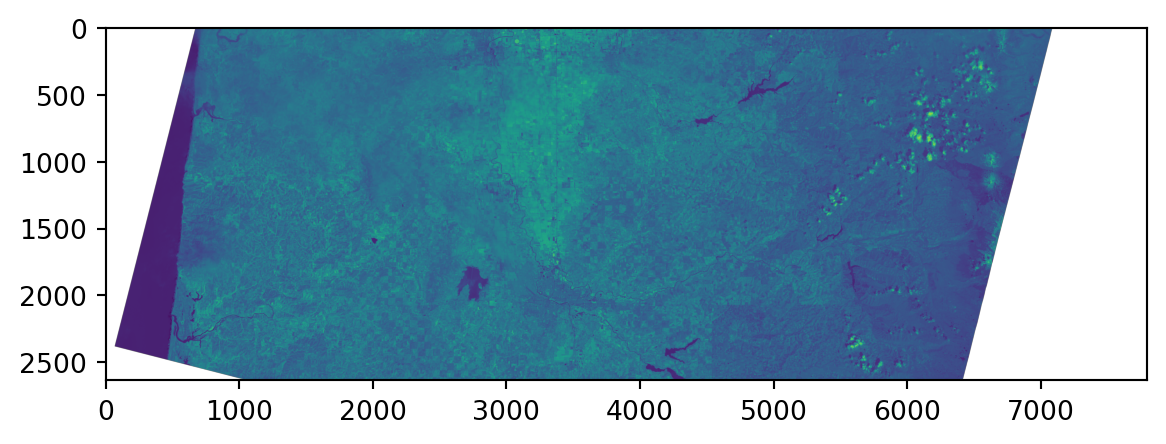
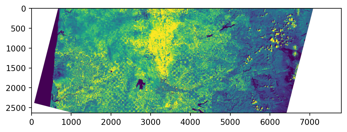
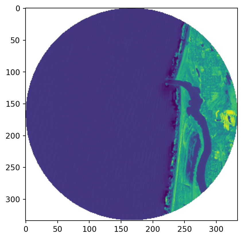
Viewing the raster:
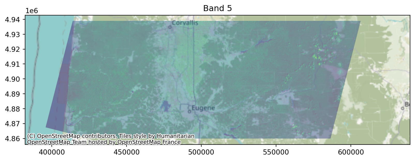
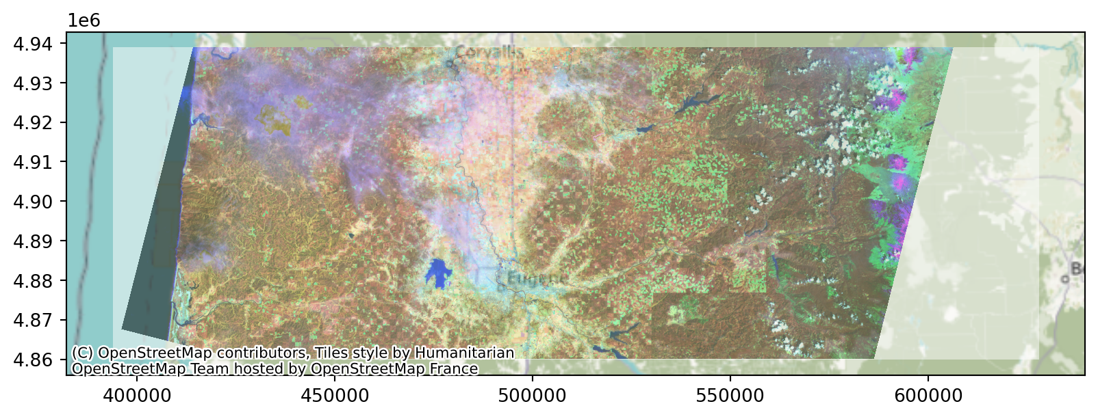
Viewing the raster, in context:
Note the crs!
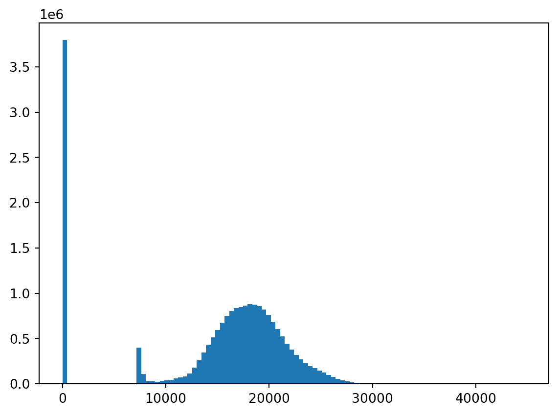
Values:
raster.read() gets a numpy array of the values. Note the missing data:
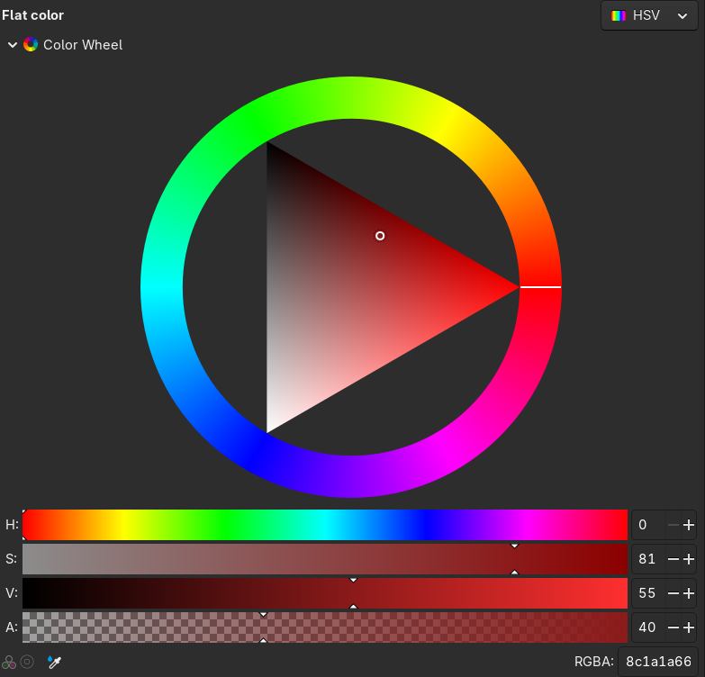
A quick reminder about “colorspace”:
- Human retinas most commonly have three kinds of color-sensitive photoreceptors.
- So, our color perception is “three-dimensional”.
- Printing: RGB (e.g., #3A11FF;) or CMYK
- Perception: HSL and HSV
- Plus: transparancy, or
alpha: #3A11FF00; - On computer monitors, RGB values range from 0 to 255.
So, by “make an image” we mean “make 1 to 3 rectangular arrays of integers between 0 and 255”.
Low contrast?

Well, that makes sense:
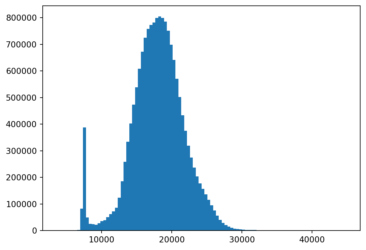
Let’s rescale!
And, let’s work with just numpy arrays for a bit.
Rescaling:
And, let’s work with just numpy arrays for a bit.
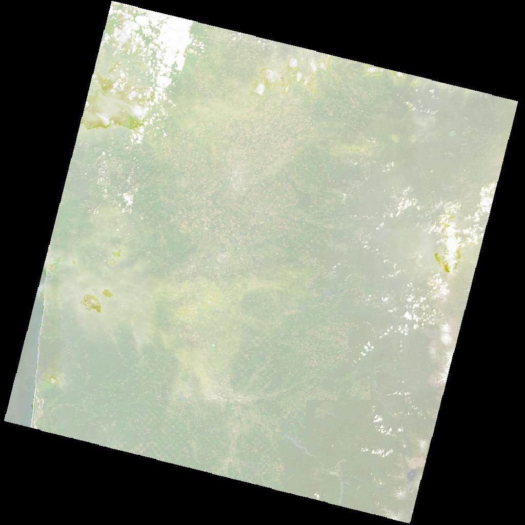
How about in color?
def norm_values(bn):
    values = bands[bn].read(masked=True)
    a, b = np.quantile(values.data[~values.mask], q=[0.05, 0.95])
    values = 255*(values - a)/(b - a)
    values[values<0] = 0
    values[values>255] = 255
    return values.astype(int)

values = np.ma.array([norm_values(bn) for bn in ["BAND_5", "BAND_6", "BAND_3"]]).squeeze()
values = np.moveaxis(values, [0, 1, 2], [2, 0, 1])
print('values:', values.shape)
plt.imshow(values);
values: (2635, 7801, 3)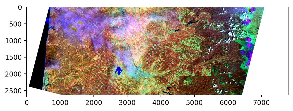
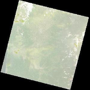
Putting this back on a map:
All it takes is the right transform argument!
Or, with ax.imshow:
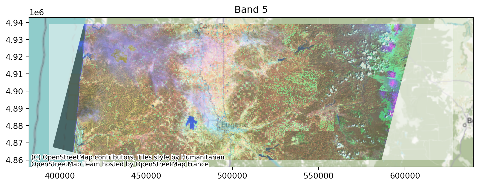
Of use: mask